Conditional Drop-Down List with IF Statement (5 Examples)
If you need to create a drop-down list that changes based on what you select in another cell, adding a condition to the drop-down list can be a helper solution. When creating a conditional drop-down list, utilizing the IF statement is an intuitive method, as it is always used to test conditions in Excel. This tutorial demonstrates 5 methods that will assist you in creating a conditional drop-down list in Excel step-by-step.
Use IF or IFS statement to create a conditional drop-down list
This section provides two functions: the IF function and the IFS function to help you create a conditional drop-down list based on other cells in Excel with two examples.
Add a single condition, like two countries and their cities
As shown in the gif below, you can easily switch between cities in two countries “United States and France” in the drop-down list. Let's see how to use an IF function to get it done.
Step 1: Create the main drop-down list
First, you need to create a main drop-down list that will serve as the basis for your conditional drop-down list.
1. Select a cell (E2 in this case) where you want to insert the main drop-down list. Go to the Data tab, select Data Validation.

2. In the Data Validation dialog box, follow these steps to configure the settings.

Step 2: Create a conditional drop-down list with an IF statement
1. Select the range of cells (In this case, E3:E6) where you want to insert the conditional drop-down list.
2. Go to the Data tab, select Data Validation.
3. In the Data Validation dialog box, you need to configure as follows.
=IF($E$2=$B$2,$B$3:$B$6,$C$3:$C$6)
Result
The conditional drop-down list is now complete.
As shown in the gif image below, if you want to select a city in United States, click on E2 to select Cities in United States from the drop-down list. Then select any city belonging to United States in the cells below E2. To select a city in France, do the same operation.
Add multiple conditions, like more than two countries and their cities
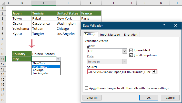
As shown in the gif image below, there are two tables. The one column table contains different countries, while the multi-column table contains cities in those countries. Here we need to create a conditional drop-down list that contains cities that will change according to the country you choose in E10, please follow the steps below to complete.
Step 1: Create a drop-down list containing all the countries
1. Select a cell (Here I select E10) where you want to display the country, go to the Data tab, click Data Validation.
2. In the Data Validation dialog box, you need to:

The drop-down list contains all countries is now complete.
Step 2: Name the cell range for the cities under each country
1. Select the entire range of the cities table, go to the Formulas tab, click Create from Selection.

2. In the Create Names from Selection dialog box, only check the Top row option and click the OK button.


Step 3: Create a conditional drop-down list
1. Select a cell (here I select E11) to output the conditional drop-down list, go to the Data tab, select Data Validation.
2. In the Data Validation dialog box, you need to:
=IF($E$10="Japan",Japan,IF(E10="Tunisia",Tunisia,IF(E10="United States",United_States, France)))
=IFS(E10="Japan",Japan,E10="Tunisia",Tunisia,E10="United States",United_States,E10="France", France)Result
Just a few clicks to create a conditional drop-down list with Kutools for Excel
The above methods might be cumbersome for most Excel users. If you want a more effecient and straightforward solution, the Dynamic Drop-down List feature of Kutools for Excel is highly recommended to help you create a conditional drop-down list with just a few clicks.
As you can see, the whole operation can be done in just a few clicks. You just need to:
A better alternative to the IF function: the INDIRECT function
As an alternative to the IF and IFS functions, you can use a combination of the INDIRECT and SUBSTITUTE functions to create a conditional drop-down list, which is simpler than the formulas we provided above.
Take the same example used in the multiple conditions above (as shown in the gif image below). Here I will show you how to use the combination of the INDIRECT and SUBSTITUTE functions to create a conditional drop-down list in Excel.
1. In cell E10, create the main drop-down list containing all countries. Follow the above step 1.
2. Name the cell range for the cities under each country. Follow the above step 2.
3. Use the INDIRECT and SUBSTITUTE functions to create a conditional drop-down list.
Select a cell (E11 in this case) to output the conditional drop-down list, go to the Data tab, select Data Validation. In the Data Validation dialog box, you need to:
=INDIRECT(SUBSTITUTE(E10," ","_"))
You have now successfully created a conditional drop-down list using the INDIRECT and SUBSTITUTE functions.
Related Articles
Autocomplete when typing in Excel drop down list
If you have a data validation drop down list with large values, you need to scroll down in the list just for finding the proper one, or type the whole word into the list box directly. If there is method for allowing to auto complete when typing the first letter in the drop down list, everything will become easier. This tutorial provides the method to solve the problem.
Create drop down list from another workbook in Excel
It is quite easy to create a data validation drop down list among worksheets within a workbook. But if the list data you need for the data validation locates in another workbook, what would you do? In this tutorial, you will learn how to create a drop fown list from another workbook in Excel in details.
Create a searchable drop down list in Excel
For a drop down list with numerous values, finding a proper one is not an easy work. Previously we have introduced a method of auto completing drop down list when enter the first letter into the drop down box. Besides the autocomplete function, you can also make the drop down list searchable for enhancing the working efficiency in finding proper values in the drop down list. For making drop down list searchable, try the method in this tutorial.
Auto populate other cells when selecting values in Excel drop down list
Let’s say you have created a drop down list based on the values in cell range B8:B14. When you selecting any value in the drop down list, you want the corresponding values in cell range C8:C14 be automatically populated in a selected cell. For solving the problem, the methods in this tutorial will do you a favor.
Best Office Productivity Tools
Supercharge Your Excel Skills with Kutools for Excel, and Experience Efficiency Like Never Before. Kutools for Excel Offers Over 300 Advanced Features to Boost Productivity and Save Time. Click Here to Get The Feature You Need The Most...
Office Tab Brings Tabbed interface to Office, and Make Your Work Much Easier
- Enable tabbed editing and reading in Word, Excel, PowerPoint, Publisher, Access, Visio and Project.
- Open and create multiple documents in new tabs of the same window, rather than in new windows.
- Increases your productivity by 50%, and reduces hundreds of mouse clicks for you every day!
All Kutools add-ins. One installer
Kutools for Office suite bundles add-ins for Excel, Word, Outlook & PowerPoint plus Office Tab Pro, which is ideal for teams working across Office apps.
- All-in-one suite — Excel, Word, Outlook & PowerPoint add-ins + Office Tab Pro
- One installer, one license — set up in minutes (MSI-ready)
- Works better together — streamlined productivity across Office apps
- 30-day full-featured trial — no registration, no credit card
- Best value — save vs buying individual add-in