Combine two columns in Excel (Step-by-step tutorial)
When working with Excel, you may encounter situations where combining two columns becomes necessary to improve data organization and facilitate your work. Whether you are creating full names, addresses, or performing data cleaning and analysis, merging columns can significantly enhance your ability to process and utilize data efficiently. In this tutorial, we will guide you through the process of combining two columns in Excel, whether you want to concatenate text, merge dates, or combine numerical data. Let's get started!

Video: Combine two columns in Excel
Combine two or multiple columns in Excel
In this section, we will explore three methods to combine two or more columns. These techniques will enable you to merge and consolidate data in Excel efficiently. Whether you need to concatenate values, or consolidate information from multiple columns, these methods have got you covered. Let's dive in and discover how to merge columns effectively in Excel.
Combine two columns using ampersand (&)
Let's assume you have first names in column A and last names in column B, and you want to combine them to create a full name in another column. To achieve this, please perform the following steps.
Step 1: Input the formula with ampersand (&)
- Select the top cell of the column where you want to combine the two columns, and input the below formula.
-
=A2&" "&B2 - Press the "Enter" key.


Step 2: Copy the formula down to below cells to get all results
Double-click on the fill handle (the small green square in the lower-right corner) of the formula cell to apply the formula to below cells.
Notes:
- You can replace the space (" ") in the formula with:
- Other separators you want, e.g., a comma (", ").
Remember to enclose the separator with quotation marks. Adding a space after the separator would improve readability. 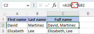
- Any text you will add between the concatenated values, e.g., is from (" is from ").
Remember to enclose the text with quotation marks, and add spaces before and after the text. 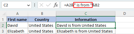
- Other separators you want, e.g., a comma (", ").
- To merge three columns, use the formula below. This pattern can be continued to merge additional columns by appending their respective references.
-
=A2&" "&B2&" "&C2 


Merge columns quickly and easily using a versatile tool
Combining data using the ampersand symbol (&) from multiple columns can be a tedious process and prone to errors, as it requires typing &" "& and selecting multiple cells repeatedly. However, with "Kutools for Excel", you can easily combine columns in just a few clicks, saving you time and effort.
Once you have selected the columns to be combined, select "Kutools" > "Merge & Split" > "Combine Rows, Columns or Cells without Losing Data", and follow the steps below:
- Select "Combine columns".
- Select a separator you need. In this example, I selected "Other separator", and entered a comma (, ).
Here we add a space after the comma to make the combined text easier to read. - Specify where you want to put the combined data.
- Select how you want to deal with the combined cells.
- Click "Ok".


Result
In addition to the ability of combining columns and placing the result in a new location, the Combine Rows, Columns or Cells without Losing Data feature provides the added functionality of directly combining the source data in place.

Note: If you do not have Kutools for Excel installed, please download and install it. The professional Excel add-in offers a 30-day free trial with no limitations.
Join two columns using Excel concatenating functions
Before we proceed with merging data from two columns into a single column using an Excel function, let's take a look at the following three commonly used functions for combining data. After that, we will dive into the step-by-step process.
| "CONCATENATE" | - | Available in all versions of Excel (may not be available in future versions). |
| "CONCAT" | - | Available in Excel 2016 and newer versions, as well as in Office 365. |
| "TEXTJOIN" | - | Available in Excel 2019 and newer versions, as well as in Office 365. The "TEXTJOIN" function provides more flexibility and efficiency than "CONCATENATE" and" CONCAT" when combining multiple columns. |
Step 1: Select a blank cell where you want to put the combined data
Here I will select the cell C2, which is the top cell of the column where I will combine the two columns.

Step 2: Input the formula
Use one of the following formulas, and then press "Enter" to get the result. (In this example, I will enter the formula with the "CONCATENATE" function.)
=CONCATENATE(A2," ",B2)=CONCAT(A2," ",B2)=TEXTJOIN(" ",TRUE,A2:B2)Step 3: Copy the formula down to below cells to get all results
Double-click on the fill handle (the small green square in the lower-right corner) of the formula cell to apply the formula to below cells.
Notes:
- You can replace the space (" ") in the formula with:
- Other separators you want, e.g., a comma (", ").
Remember to enclose the separator with quotation marks. Adding a space after the separator would improve readability. 
- Any text you want to add between the concatenated values, e.g., is from (" is from ").
Remember to enclose the text with quotation marks, and add spaces before and after the text. 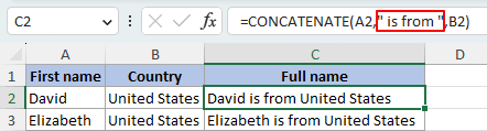
- Other separators you want, e.g., a comma (", ").
- To combine three columns, use any of the formulas below. Note that this pattern can be extended to merge additional columns by appending their respective references.
-
=CONCATENATE(A2," ",B2," ",C2)=CONCAT(A2," ",B2," ",C2)=TEXTJOIN(" ",TRUE,A2:C2) 
- For users of Excel 2019 or later versions who want to "combine more than three columns", I recommend using the "TEXTJOIN" function, since which allows you to combine cell values by selecting a whole range of values instead of repeatedly typing delimiters and selecting each cell individually.


Combine columns containing formatted numbers (dates, currency, …)
Suppose you need to merge two columns, one of which contains formatted numbers. If you use a regular formula we talked above, the formatting of the numbers will be lost and you'll end up with the following results.

This is why it's important to format combined columns properly, especially when they contain a mix of text, numbers, dates, and other data types. To correctly display formatted numbers when concatenating, here are three methods you can follow.
Correctly display formatted numbers with TEXT function
In this section, I'll show you how to use the "TEXT" function to preserve the correct number formatting, and then combine the columns using the "ampersand method "as an example. Keep in mind that you can apply the same technique to the" concatenating functions method" as well.
Step 1: Select the formula that suits your data type
To combine Column 1 (text) and Column 2 (differently formatted numbers) in the example above while retaining their formatting, we can use the "TEXT" function to customize the display of the numbers. Below are the formulas that can be used to combine text with the formatted numbers mentioned above. You can simply copy the formula that suits your requirements.
| Formatted number | Data type of formatted number | Formula |
|---|---|---|
| 5/12/2023 | Date (Month/Day/Year with no leading zeros) | =A2&" "&TEXT(B2,"m/d/yyyy") |
| 4:05:00 PM | 12-hour time format with AM/PM (Hours with no leading zeros, Minutes and Seconds with leading zeros) | =A3&" "&TEXT(B3,"h:mm:ss AM/PM") |
| 1000.00 | Number with 2 decimal places | =A4&" "&TEXT(B4,"#.00") |
| $1,000 | Currency with a thousand separator | =A5&" "&TEXT(B5,"$#,##0") |
| 11.1% | Percentage with 1 decimal place | =A6&" "&TEXT(B6,"#.0%") |
| 1/2 | Fraction | =A7&" "&TEXT(B7,"#/#") |
Result
By utilizing the formulas mentioned above, you will be able to obtain the combined results with correctly displayed formatted numbers.

Note:
If you cannot find a format that matches your requirements from the above table, you can create a custom format code to replace the existing one, such as "m/d/yyyy", within the "TEXT" function.
For example, to combine a text column with a column containing numbers that use a comma as a thousands separator, change the formula =A2&" "&TEXT(B2,"m/d/yyyy") to =A2&" "&TEXT(B2,"#,###").
Please visit this page for more information on creating a custom format code.
Correctly display formatted numbers with Kutools' Use Formatted Values option
The "Combine Rows, Columns or Cells without Losing Data" feature offers a "Use Formatted Values" option. By selecting this option, you can easily combine text and formatted numbers while correctly displaying their formatting without typing any formulas.
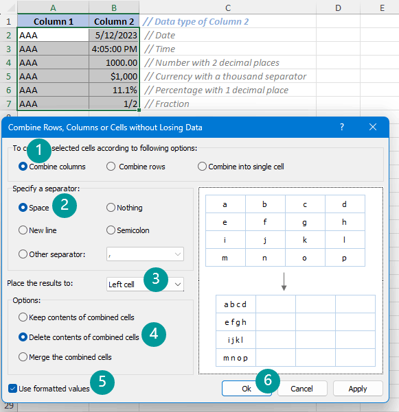
After selecting the columns that you wish to combine, proceed to select "Kutools" > "Merge & Split" > "Combine Rows, Columns or Cells without Losing Data", and follow the steps below:
- Select "Combine columns".
- Select a separator you need. In this example, I selected "Space".
- Specify where you want to put the combined data.
- Select how you to want to deal with the combined cells.
- Check the "Use formatted values" option.
- Click "Ok".

Result
The Combine Rows, Columns or Cells without Losing Data feature not only allows you to merge columns and store the result in a different location like other methods do, but it also enables you to directly merge the original data in place without losing any formatting.

Note: If you do not have Kutools for Excel installed, please download and install it. The professional Excel add-in offers a 30-day free trial with no limitations.
Correctly display formatted numbers with Notepad
The Notepad method is an alternative approach to combine columns with formatted numbers, although it may involve a few additional steps. Once you become familiar with the process, it can be a fast and convenient method for combining data, especially when compared to using formulas.
Note: The method is suitable for combining adjacent columns only.
Step 1: Copy the columns to be combined
Select the columns and press "Ctrl" + "C" to copy them.

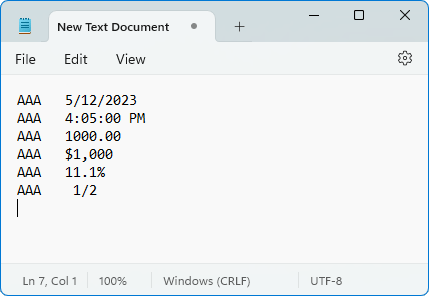
Step 2: Paste the copied columns to Notepad
- Press "Windows key" + "S", type "Notepad", then select "Notepad" from the results.

- In the "Notepad" window, press "Ctrl" + "V" to paste the copied columns.


Step 3: Replace separator in Notepad with the one you need
- Select the separator between the column values, then press "Ctrl" + "C" to copy it.
- Press "Ctrl" + "H" to open the "Find and Replace" dialog box, and then press "Ctrl" + "V" to paste the copied separator to the "Find what" box.
- Enter the separator you need in the "Replace with" box. In this example, I entered a space ( ).
- Click "Replace all".


Step 4: Copy the combined result to Excel sheet
- To copy all the text in Notepad, press "Ctrl + A" to select everything, and then press "Ctrl + C" to copy the selected text.
- Go back to your Excel worksheet, select the top cell of the desired location where you will put the combined result, and then press "Ctrl + V" to paste the copied text.


Result

Optional: Convert formula-combined results to static values
The combined column you created using the formula methods will be dynamic, which means that any changes in the original values will affect the values in the combined column. Additionally, if any of the source columns are deleted, the corresponding data in the combined column will also be removed. To prevent this, please do as follows.
Step 1: Convert formula to value
Select the values you combined using formulas, then press "Ctrl" + "C". Next, right-click on any of the selected cells, and select the "Values" button from "Paste Options".

Result
By doing this, you will paste only the values, removing the formulas. The combined values will become static and will not be affected by future changes in the original data.

Best Office Productivity Tools
Supercharge Your Excel Skills with Kutools for Excel, and Experience Efficiency Like Never Before. Kutools for Excel Offers Over 300 Advanced Features to Boost Productivity and Save Time. Click Here to Get The Feature You Need The Most...
Office Tab Brings Tabbed interface to Office, and Make Your Work Much Easier
- Enable tabbed editing and reading in Word, Excel, PowerPoint, Publisher, Access, Visio and Project.
- Open and create multiple documents in new tabs of the same window, rather than in new windows.
- Increases your productivity by 50%, and reduces hundreds of mouse clicks for you every day!
All Kutools add-ins. One installer
Kutools for Office suite bundles add-ins for Excel, Word, Outlook & PowerPoint plus Office Tab Pro, which is ideal for teams working across Office apps.
- All-in-one suite — Excel, Word, Outlook & PowerPoint add-ins + Office Tab Pro
- One installer, one license — set up in minutes (MSI-ready)
- Works better together — streamlined productivity across Office apps
- 30-day full-featured trial — no registration, no credit card
- Best value — save vs buying individual add-in
Table of contents
- Combine two or multiple columns in Excel
- With ampersand (&)
- With a versatile tool
- With Excel concatenating functions
- Combine columns containing formatted numbers (dates, currency, …)
- With TEXT function
- With Kutools’ Use Formatted Values option
- With Notepad
- Optional: Convert formula-combined results to static values
- Related articles
- The Best Office Productivity Tools
- Comments