Find highest value in Excel (Step-by-step guide)
Finding the highest value in Excel is a common task when working with numerical data. Whether you need to identify the largest number within a set of values or determine the position of the highest value, the tutorial provides several functions and techniques to help you accomplish this.
 |
Video: Find highest value in Excel
Return highest value in Excel
In this section, we will talk about two easy methods to evaluate the values in a specified range and return the largest value among them.
Get highest value with MAX function
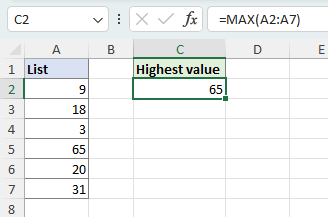
To get the highest value in the list A2:A7 by using the MAX function, please do as follows.
- Select a blank cell.
- Enter the below MAX formula, and press Enter key to get the result.
-
=MAX(A2:A7) 
- Tip: To obtain the Nth greatest number, you can utilize the LARGE function. For example, to find the 3rd largest number in the range A2:A7, use the formula below.
=LARGE(A2:A7,3)
Get highest value with AutoSum feature
To get the highest value in the list A2:A7 with AutoSum, follow the instructions below.
Note: The AutoSum function requires the numbers, from which the highest value is to be extracted, to be arranged in adjacent cells.
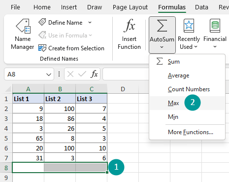
Step 1: Select a cell below or to the right of the numbers from which to get the highest value
- To get the largest number in a column, such as in our example below, select the cell right below the numbers (cell A8 in this example).
- To get the largest number in a row, select the cell to the right of numbers.

Step 2: Select AutoSum > Max
On the "Formulas" tab, in the "Function Library" group, click the arrow below "AutoSum", and select "Max".

Step 3: Press Enter to get the greatest value
A MAX formula is automatically generated with the numbers selected, as shown in the picture on the left. Press Enter to execute the formula, and you will get the highest value among the selected numbers, as shown in the picture on the right.

Tips:
- The AutoSum function is especially useful when dealing with long contiguous rows or columns, as it eliminates the need for manual selection or typing the range in a MAX formula.
- If dealing with multiple columns or rows, select cells at the bottom or right of your table, then click "AutoSum" > "Max" to find the highest value for each column or row simultaneously.

Find maximum value in Excel
In this section, I will introduce ways to either highlight, selector locatethe highest value among a group of numbers, so that you can easily identify and work with the maximum value in your Excel data.
Highlight all greatest values with Conditional Formatting
Conditional formatting allows us to apply visual cues to cells based on specific conditions or criteria. In this section, we will learn how to use conditional formatting in Excel to highlight all cells containing the maximum value within a range.
Step 1: Select the range from which to find the highest value

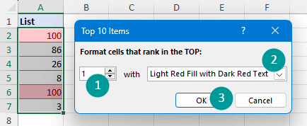
Step 2: On the "Home" tab, select "Conditional Formatting" > "Top/Bottom Rules" > "Top 10 Items".

Step 3: Set conditional formatting rule
- Enter "1" in the input box to format only the cells with the highest value.
- Choose your preferred formatting option from the predefined options or customize your own format by selecting "Custom Format...."
- Once finished setting, click OK. Any changes you make in the dialog box are instantly reflected in your dataset, providing a preview of the final appearance once you hit OK.

Select highest values within ranges, columns, or rows with Kutools
Kutools for Excel's "Select Cells with Max & Min Value" feature allows you to select the largest value in a specified range, or select the highest values across each column/row within that range. Moreover, it provides the versatility to either select the first instance of the highest value or select all cells that contain the peak value.
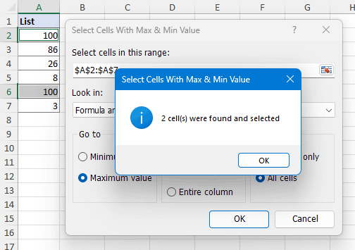
After installing Kutools for Excel, select the range for which to find the highest value, then click "Kutools" > "Select" > "Select Cells with Max & Min Value", and do as follows:

- Specify the type of cells within the selected range to search for max values in the "Look in" drop-down list: "Formula and Value Cells", "Formula Cells Only", or "Value Cells Only". Here I selected Formula and Value Cells.
- Select "Maximum value" in the "Go to" section.
- Select "Cell" in the "Base" section.
- Select "All cells" in the "Select" section.
Result
The cells with the highest value are instantly selected, and a dialog box displays the number of cells that were found and selected.
Note: To enable this feature, please download and install Kutools for Excel.
Get cell address of highest value with Excel functions
- To get the cell address of the maximum value in a column (Column A in the example), use the below formula.
-
=ADDRESS(MATCH(MAX(A:A),A:A,0),COLUMN(A:A)) If your numbers are in another column, modify the formula by replacing "A:A" with the corresponding column reference.
Formula breakdown:
- MAX(A:A): Finds the maximum value among the numbers in column A, which is 65.
- MATCH(MAX(A:A),A:A,0) = MATCH(65,A:A,0): Returns the position of the maximum value 65 in column A, which is 5.
- COLUMN(A:A): Returns the column number of column A, which is 1.
- ADDRESS(MATCH(MAX(A:A),A:A,0),COLUMN(A:A)) = ADDRESS(5,1): Returns the cell address based on the given specified row and column numbers, which is $A$5.

- To get the cell address of the maximum value in a row (Row 1 in the example), use the below formula.
-
=ADDRESS(1,MATCH(MAX(1:1),1:1,0)) If your numbers are in another row, replace all the "1"s in the formula with the corresponding row number.
Formula breakdown:
- MAX(1:1): Finds the maximum value among the numbers in row 1, which is 65.
- MATCH(MAX(1:1),1:1,0) = MATCH(65,1:1,0): Returns the position of the maximum value 65, in row 1 - which is located in the fifth column.
- ADDRESS(1,MATCH(MAX(1:1),1:1,0)) = ADDRESS(1,5): Returns the cell address based on the given specified row and column numbers, which is $E$1.

Note: If there are multiple occurrences of the highest number, the formula will only provide the cell address of the first instance.
Above is all the relevant content related to finding the highest value in Excel. I hope you find the tutorial helpful. If you're looking to explore more Excel tips and tricks, please click here to access our extensive collection of over thousands of tutorials.
Related articles
- How to find the lowest and highest 5 values in a list in Excel?
- For a list of score in Excel, you may need to identify the highest and lowest 5 values in order to have a comparison among them. With this tutorial, you will learn how to find the lowest and highest 5 values in a list.
- How to find the highest value and return adjacent cell value in Excel?
- If you have a range of data as following screenshot shown, now, you want to find the largest value in column A and get its adjacent cell content in column B. In Excel, you can deal with this problem with some formulas.
- How to find highest value in a row and return column header in Excel?
- In this article, I will talk about how to return the column header of the largest value in a row in Excel. For Example, I have the following data range, column A is the year, and column B to F are populated the order numbers from Jan to May. And now, I want to get the month name of the largest value in each row.
- How to display the highest score and its corresponding name in Excel?
- Supposing, I have range of data which contains two columns – name column and the corresponding score column, now, I want to get the name of the person who scored highest. Are there any good ways to deal with this problem quickly in Excel?
Best Office Productivity Tools
Supercharge Your Excel Skills with Kutools for Excel, and Experience Efficiency Like Never Before. Kutools for Excel Offers Over 300 Advanced Features to Boost Productivity and Save Time. Click Here to Get The Feature You Need The Most...
Office Tab Brings Tabbed interface to Office, and Make Your Work Much Easier
- Enable tabbed editing and reading in Word, Excel, PowerPoint, Publisher, Access, Visio and Project.
- Open and create multiple documents in new tabs of the same window, rather than in new windows.
- Increases your productivity by 50%, and reduces hundreds of mouse clicks for you every day!
All Kutools add-ins. One installer
Kutools for Office suite bundles add-ins for Excel, Word, Outlook & PowerPoint plus Office Tab Pro, which is ideal for teams working across Office apps.
- All-in-one suite — Excel, Word, Outlook & PowerPoint add-ins + Office Tab Pro
- One installer, one license — set up in minutes (MSI-ready)
- Works better together — streamlined productivity across Office apps
- 30-day full-featured trial — no registration, no credit card
- Best value — save vs buying individual add-in
Table of contents
- Video: Find highest value in Excel
- Return highest value in Excel
- By MAX function
- By AutoSum feature
- Find maximum value in Excel
- Highlight all max values with Conditional Formatting
- Select highest values in a ranges, each column, or each row with Kutools
- Get cell address of highest value with Excel functions
- Related articles
- The Best Office Productivity Tools
- Comments
