8 Ways to Insert a Check Mark (Tick Symbol √) in Excel
One of the many symbols you might find yourself using regularly when working with Excel is the check mark. The check mark or tick symbol (√) is an essential tool for visually indicating completion, approval, or positive attributes. However, one may find it a bit tricky to insert symbols such as the check mark (tick symbol √) in Excel. In this article, we will explore various methods to insert a check mark in Excel.
Check Mark Vs Check Box
Before we delve into the methods of inserting a check mark, let us distinguish it from a related element - the check box.
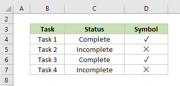
Check Mark: A check mark (√) in Excel is a static symbol. It is used to indicate that a task, item, or condition has been completed or verified. You can directly insert it into a cell. Once inserted, it becomes part of the data within the cell and remains constant unless manually edited.
The opposite of a check mark is a cross mark (x), indicating that a task, item, or condition has not been completed or verified.Check Box: Conversely, a check box is a dynamic, interactive tool. Users can interact with a check box, checking or unchecking it to make binary choices (true/false, yes/no). It does not sit within a cell but instead hovers on top of your worksheet cells as an overlaid object. If you want to know how to insert check box in Excel, please see Excel Checkboxes.

Insert a Check Mark (Tick Symbol √) in Excel
Now, let us go through the various methods you can use to insert a check mark into an Excel cell.
Using the Symbol Command to Insert a Check Mark
The most straightforward way to insert a check mark is through the "Symbol" command.
Step 1: Select the cell where you want to insert the tick symbol

Step 2: Navigate to the Insert tab and click Symbol

Step 3: In the Symbol dialog box, follow these steps:
1. Select "Wingdings" from the "Font" drop-down menu;
2. Scroll down to find the check mark. A few tick symbols and cross symbols can be found at the bottom of the list;

Tip: Alternatively, you can enter 252 into the "Character code " box at the bottom of the "Symbol "dialog to find the check mark, or enter 251 to find the cross mark.
3. Select the symbol you want. Click "Insert" to insert the symbol and click "Close" to close the Symbol window.
In this case, I select the check mark (√) to insert.

Tip: Apart from clicking the "Insert" button to insert the symbol, you can also "double-click" on the symbol itself to add it to the selected cell.
Result

🌟 Reuse Check Marks with Ease! 🌟
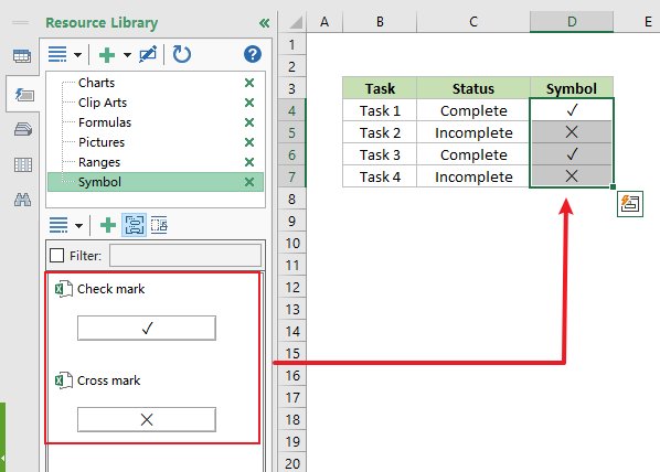
Save time and effort with Kutools for Excel's Resource Library utility! 🚀
Forget the hassle of searching for check mark symbols in the Symbol dialog box. With our "Resource Library" feature, you can save check mark and cross mark symbols as entries, allowing you to reuse them effortlessly with just one click in any workbook. Simplify your Excel experience! 💪
📊 Kutools for Excel: Your Time-Saving Excel Companion 🚀
Download NowUsing Copy and Paste to Insert a Check Mark
If the check mark symbol is already available in another cell, document, or webpage, you can simply copy and paste it into Excel. Since you're currently engaged with this article, you can conveniently copy the check mark or cross mark provided below and use it in your Excel spreadsheet.
Follow the steps below to add a check mark to your Excel sheet.
1. Select one of the symbols below. Here I select a check mark. And press the Ctrl + C keys to copy it.
| Symbol |
|---|
| ☑ |
| ☒ |
| ☓ |
| ✅ |
| ✓ |
| ✔ |
| ✕ |
| ✖ |
| ✗ |
| ✘ |
| ❌ |
| ❎ |
2. Then, select the cell where you want to paste the checkmark. Then press Ctrl + V to paste the checkmark.

Batch Insert Check Marks Quickly Using Kutools
Kutools for Excel offers the "Insert Bullet" feature, which allows you to batch insert check marks into multiple cells in few clicks, thereby saving time, especially when working with large datasets. Unlike Excel's built-in Symbol function, this feature eliminates the need to change fonts. It also supports batch insertion of other symbols, offering enhanced customization options for your data.
After selecting the cells where you want to insert check marks, click "Kutools" > "Insert" > "Insert Bullet". A list of symbols will appear. Click on the check mark symbol and it will be inserted in all the selected cells.

Tip: To use this feature, you should install Kutools for Excel first, please click to download now.
Using the Character Code to Insert a Check Mark
Excel allows inserting symbols using their specific character codes. To insert a tick symbol, simply hold the "Alt" key and type the corresponding character code. Detailed steps for this method are as follows.
Step 1: Select the cell where you want to insert the check mark
Step 2: Change the font
Go to the "Home" tab, then in the "Font" group, change the font to "Wingdings".

Step 3: Use character code to inset check mark
Press and hold the "Alt" key while using the numeric keypad to type one of the following character codes. In this case, to insert a tick symbol (√), type 0252 while holding the "Alt" key.
| Symbol name | Symbol | Character code |
|---|---|---|
| Cross symbol |  | Alt+0251 |
| Tick symbol |  | Alt+0252 |
| Cross in a box |  | Alt+0253 |
| Tick in a box |  | Alt+0254 |
Result
Release the "Alt" key and the check mark now appears in the selected cell.

Tip: To successfully use character codes, make sure to turn on NUM LOCK and utilize the numerical keypad on the keyboard instead of the QWERTY numbers above the letters.
Using the UNICHAR Function to Insert a Check Mark
While both the CHAR and UNICHAR functions can be used for inserting check marks in Excel, there are two significant limitations of the CHAR function:
- Users have to change the font to "Wingdings" to obtain the desired symbol.
- And even worse, the CHAR function in Excel 365 may not consistently display the check mark symbol (√) as expected, even when using "Wingdings" or other symbol fonts.
To ensure reliable and consistent results when inserting symbols like the check mark (√) in Excel, it is recommended to use the UNICHAR function, which returns the Unicode character or symbol based on the Unicode number provided.
To insert a check mark using the UNICHAR function in Excel, follow these steps:
Step 1: Select the cell where you want to insert the check mark
Step 2: Input the UNICHAR formula
Select one of the following formulas to insert the symbol accordingly.
| Symbol name | Symbol | Unicode | Formula |
|---|---|---|---|
| Ballot Box With Check | ☑ | 9745 | =UNICHAR(9745) |
| Ballot Box With X | ☒ | 9746 | =UNICHAR(9746) |
| St. Andrew's Cross | ☓ | 9747 | =UNICHAR(9747) |
| White Heavy Check Mark |  | 9989 | =UNICHAR(9989) |
| Check Mark | ✓ | 10003 | =UNICHAR(10003) |
| Heavy Check Mark | ✔ | 10004 | =UNICHAR(10004) |
| Multiplication X | ✕ | 10005 | =UNICHAR(10005) |
| Heavy Multiplication X | ✖ | 10006 | =UNICHAR(10006) |
| Ballot X | ✗ | 10007 | =UNICHAR(10007) |
| Heavy Ballot X | ✘ | 10008 | =UNICHAR(10008) |
| Cross Mark |  | 10060 | =UNICHAR(10060) |
| Negative Squared Cross Mark |  | 10062 | =UNICHAR(10062) |
| Diagonal X | ⨯ | 10799 | =UNICHAR(10799) |
| Circled X | ⮾ | 11198 | =UNICHAR(11198) |
| Heavy Circled X | ⮿ | 11199 | =UNICHAR(11199) |
In this case, to insert a check mark (√), enter the below formula and press Enter to get the result.
=UNICHAR(10003)Result

Using the Keyboard Shortcuts to Insert a Check Mark
Another way to insert a check mark in Excel is using keyboard shortcut. By applying either the "Wingdings 2" or "Webdings" fonts to your selected cells, you can use the corresponding keyboard shortcuts to insert different styles of check marks or cross marks.
To insert a check mark using this method, detailed steps are as follows.
Step 1: Select the cell where you want to insert the check mark
Step 2: Change the font
Go to the "Home" tab, then in the "Font" group, change the font to "Wingdings 2" or "Webdings". In this case, I choose font "Webdings".

Step 3: Press the corresponding keyboard shortcut to insert check mark
| Wingdings 2 | Webdings | ||
|---|---|---|---|
| Symbol | Shortcut | Symbol | Shortcut |
 | Shift + P |  | a |
 | Shift + R |  | r |
 | Shift + O | ||
 | Shift + Q | ||
 | Shift + S | ||
 | Shift + T | ||
 | Shift + V | ||
 | Shift + U | ||
In this case, to insert the check mark, press the a key.
Result

Using AutoCorrect to Insert a Check Mark
You can configure Excel's "AutoCorrect" feature to automatically replace a specific text string with a check mark symbol. Once this is set up, each time you input this specific text, Excel will automatically replace it with a check mark symbol. Let's explore this method now!
Step 1: Set up AutoCorrect in Excel
1. Select one of the symbols below. Here I select a check mark. And press the "Ctrl + C" keys to copy it.
| Symbol |
|---|
| ☑ |
| ☒ |
| ✓ |
| ✔ |
| ✕ |
| ✖ |
2. Click on the "File" tab, then click "Options".
3. In the "Excel Options" dialog box, click "Proofing" and then "AutoCorrect Options".

4. In the "AutoCorrect" dialog box, please do as follows:
- In the "Replace" field, enter a word or phrase that you want to associate with the check mark symbol, such as "tick".
- In the "With" field, press "Ctrl + V" to paste the check mark symbol that you previously copied.
- Click "Add" to set the new AutoCorrect rule.
- Click OK to close the AutoCorrect dialog box.

5. Click OK close the Excel Options dialog box.
Step 2: Use AutoCorrect to insert a check mark
Now that the AutoCorrect rule is established, you simply need to type "tick" in a cell and press Enter . Then the text will automatically be replaced with a check mark.

Display Check Marks Based on Cell Values using Conditional Formatting
Conditional formatting in Excel is a versatile feature that instructs cells to behave in a certain way, depending on specific conditions. By applying conditional formatting, you can dynamically insert icons, such as check marks, based on the values in cells. Therefore, it is an effective tool for automatically displaying check marks based on a cell's value, enhancing the visual representation of your data.
In the provided data below, we aim to display a check mark when a value reaches or exceeds 3000, and a cross mark when it falls below 3000in the cell range D4:D15. Please follow the steps below to achieve this.

Step 1: Copy and paste the cells with values that you want to represent with symbols.
Here I copied values in cells C4:C15 and pasted them to cells D4:D15.

Step 2: Select the newly pasted cells where you intend to display the symbols.
Step 3: Go to the Home tab and click Conditional Formatting > Icon Sets > More Rules.

Step 4: In the New Formatting Rule dialog box, please do as follows:
1. In the "Format all cells based on their values" section, check the "Show Icon only" box. This will ensure that only the icons are visible in the selected cells, and the numbers within them remain hidden.

2. In the "Display each icon according to these rules" section, specify as follows:
- For the first icon, change it to check mark, choose "Number" from the "Type" drop-down list, and input 3000 in the "Value" box;
- For the second icon, change it to cross mark, choose "Number" from the "Type" drop-down list, and input 0 in the "Value" box;
- For the third icon, change it to "No Cell" Icon.

3. Click OK to apply the conditional formatting.
Result
Cells with values 3000 and above will show a check mark, and cells with values less than 3000 will show a cross mark.

In conclusion, there are many ways to insert a checkmark in Excel. It's up to you to choose the method that suits your needs best. If you're looking to explore more Excel tips and tricks, please click here to access our extensive collection of over thousands of tutorials.
Related articles
How to insert bullet points in text box or specify cells in Excel?
This tutorial is talking about how to insert bullet points in a text box or multiple cells in Excel.
How to insert/apply bullets and numbering into multiple cells in Excel?
Apart from copying the bullets and numbering from Word documents to workbook, the following tricky ways will help you apply the bullets and numbering in cells of Excel quickly.
How to quickly insert multiple checkboxes in Excel?
How can we quickly insert multiple check boxes in Excel? Please follow these tricky methods in Excel:
How to add check mark in a cell with double clicking in Excel?
This article will show you a VBA method to easily add check mark in a cell with double clicking only.
The Best Office Productivity Tools
Kutools for Excel - Helps You To Stand Out From Crowd
Kutools for Excel Boasts Over 300 Features, Ensuring That What You Need is Just A Click Away...
Office Tab - Enable Tabbed Reading and Editing in Microsoft Office (include Excel)
- One second to switch between dozens of open documents!
- Reduce hundreds of mouse clicks for you every day, say goodbye to mouse hand.
- Increases your productivity by 50% when viewing and editing multiple documents.
- Brings Efficient Tabs to Office (include Excel), Just Like Chrome, Edge and Firefox.
Table of contents
- Check Mark Vs Check Box
- Insert Check Mark (Tick Symbol √) in Excel
- Using the Symbol Command
- Using Copy and Paste
- Batch Insert Check Marks Quickly Using Kutools
- Using the Character Code
- Using the UNICHAR Function
- Using the Keyboard Shortcuts
- Using AutoCorrect
- Display Check Marks Based on Cell Values
- Related articles
- The Best Office Productivity Tools