How to total a column in Excel (7 methods)

Excel is a staple tool for anyone managing data. Whether you're a seasoned professional or a beginner, totaling columns is a fundamental skill you'll frequently need. It's particularly useful in scenarios like financial budgeting, sales analysis, or inventory tracking, where summing up values is essential.

For a quick glance at the sum of a column, simply select the column containing your numbers and observe the sum displayed on the status bar in the lower right corner of the Excel window.

However, if you require the sum to be displayed within your Excel spreadsheet, this guide offers the following practical approaches:

• Using the AutoSum command
• Using the SUM function
• Using shortcut keys
• Using named ranges
• By converting your data into an Excel table

• Summing only filtered (visible) cells in a column
• Conditional summing based on criteria

Total a column using the AutoSum command

AutoSum is a quick and user-friendly feature in Excel, designed to calculate the sum of a column or row with a single click. This feature is particularly useful for those who prefer not to memorize or manually type formulas.

1. Select the empty cell immediately below the numbers you need to sum.
2. Go to the "Home" tab, and in the "Editing" group, click on the "AutoSum" button.
3. Excel will automatically insert the SUM function and pick the range with your numbers. Press "Enter" to sum up the column.

   

Sum a column using the SUM function

The SUM function is a fundamental and versatile formula in Excel, allowing for precise control over which cells are totaled. It’s ideal for users comfortable with typing formulas and needing flexibility.

1. Click on the cell where you want the total to appear.
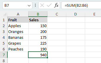
2. Type =SUM(, and then select the range of cells you want to total. For instance, based on our example, the following formula would be displayed in the formula bar:

   =SUM(B2:B6

   

   Tip: If you're working with a very long column, you can manually enter the range in the SUM function, e.g., "=SUM(B2:B500)". Alternatively, after typing =SUM(, you can select the first number in your column, and then press "Ctrl" + "Shift" + "↓" (Down Arrow) to quickly select the entire column.
3. Press "Enter" to display the total.

   

=SUM(A1, A3, A5:A10)

Add up a column using shortcut keys

The shortcut "ALT" + "=" is a swift method for summing a column, combining the convenience of AutoSum with the speed of keyboard shortcuts. It’s ideal for users who prefer keyboard shortcuts for efficiency.

1. Select the empty cell immediately below the numbers you need to sum.
2. Press "ALT" + "=".
3. Excel automatically selects the adjacent upward cells to sum. Press "Enter" to confirm the selection and calculate the total.

   

Get total of a column using named ranges

In Excel, using named ranges to add up a column simplifies your formulas, making them easier to understand and maintain. This technique is particularly valuable when dealing with large datasets or complex spreadsheets. By assigning a name to a range of cells, you can avoid the confusion of cell references like "A1:A100" and instead use a meaningful name like "SalesData". Let's explore how to effectively utilize named ranges for summing up a column in Excel.

1. Select the range of cells you want to sum.
2. Assign a name to the chosen range by typing it into the "Name Box" and pressing "Enter".

   

3. Click on the cell where you want the total of the named range to appear.
4. Enter the SUM formula using the named range. For instance, if your named range is labeled "sales", the formula would be:

   =SUM(sales)

5. Press "Enter" to display the total.

   

Total a column by converting your data into an Excel table

Excel tables are not just about organizing your data neatly. They come with a plethora of benefits, especially when it comes to performing calculations like summing up a column. This method is particularly useful for dynamic datasets where rows are frequently added or removed. By converting your data into an Excel table, you ensure that your sum calculations automatically update to include any new data added.

1. Click on any cell within your dataset.
2. Press "Ctrl" + "T".
3. In the "Create Table" dialog box, confirm the range of your data and check the box if your table has headers. Then, click "OK".

   

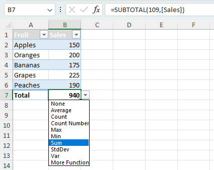
4. Click on any cell in the column you want to sum, on the "Table Design" tab, check the "Total Row" checkbox.

   

5. A total row will be added at the bottom of your table. To make sure you get the sum, choose the number in the new row and click the small arrow beside it. Then select the "Sum" option from the dropdown menu.

   

Customized approaches to summing a column

Excel offers a range of functionalities for more tailored data analysis needs. In this section, we delve into two specialized methods for summing a column: summing only filtered (visible) cells and conditional summing based on specific criteria.

Summing only filtered (visible) cells in a column

When working with large datasets, often you filter out rows to focus on specific information. However, using the standard SUM function on a filtered column might return the total of all rows, including those hidden by filters. To sum only the visible cells:

Step 1: Apply filters to a column to show only the data you need to total

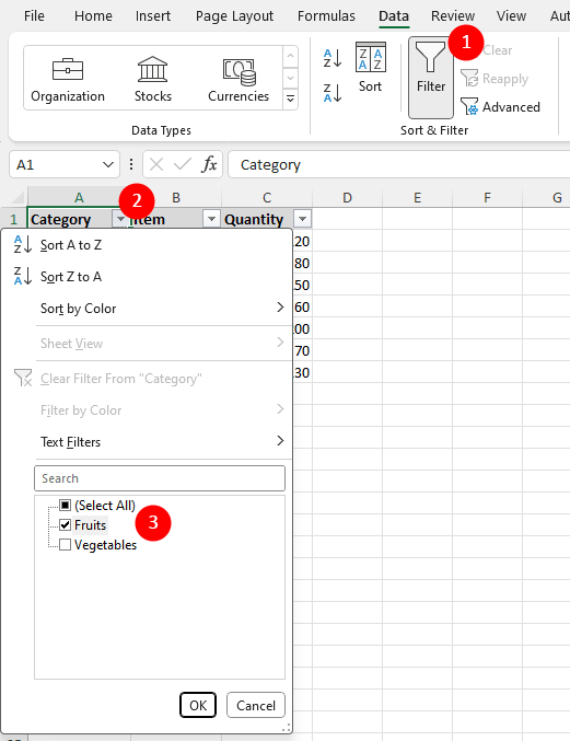
1. Click on any cell within your data, then go to the "Data" tab and click on the "Filter" button. Tip: After clicking, you will notice that the button appears pressed.
2. Click the dropdown arrow in the header of the column you wish to filter.
3. In the dropdown menu, deselect "Select All". Then, choose the specific value(s) you want to filter by. Click "OK" to apply these filters and update your data view.

   

Step 2: Use the "AutoSum" command

1. Select the empty cell immediately below the numbers you need to sum.
2. Go to the "Home" tab, and in the "Editing" group, click on the "AutoSum" button.
3. Excel will automatically insert the SUBTOTAL function and pick the visible numbers within your column. Press "Enter" to sum only the visible numbers.

   

Conditional summing based on criteria

The SUMIF function in Excel is a robust formula that provides the ability to sum cells that meet a specific condition. In this section, we'll use an example to demonstrate how to calculate the total quantity of fruits using the SUMIF function.

1. Click on the cell where you want the conditional sum to be displayed.
2. Enter the following formula.

   =SUMIF(A2:A8, "Fruits", C2:C8)

   Tip: This formula sums the values in the range "C2:C8" where the corresponding cells in the range "A2:A8" are labeled as "Fruits".

   

=SUMIFS(C2:C8, A2:A8, "A", B2:B8, "Apple")

Above is all the relevant content related to totaling a column in Excel. I hope you find the tutorial helpful. If you're looking to explore more Excel tips and tricks, please click here to access our extensive collection of over thousands of tutorials.

Related articles

• How to calculate cumulative sum / running total of a column in Excel?
• How to sum values in same column across multiple sheets?
• How to sum or count first n values in an Excel column or row?
• How to sum cells when value changes in another column?