Creating a loan amortization schedule in Excel can be a valuable skill, allowing you to visualize and manage your loan repayments effectively. An amortization schedule is a table that details each periodic payment on an amortizing loan (typically a mortgage or car loan). It breaks down each payment into interest and principal components, showing the remaining balance after each payment. Let's dive into a step-by-step guide to create such a schedule in Excel.

What is an amortization schedule?

Create an amortization schedule in Excel

Create an amortization schedule for a variable number of periods

Create an amortization schedule with extra payments

Create an amortization schedule (with extra payments) by using Excel template

What is an amortization schedule?

An amortization schedule is a detailed table used in loan calculations that displays the process of paying off a loan over time. Amortization schedules are commonly used for fixed-rate loans such as mortgages, car loans, and personal loans, where the payment amount remains constant throughout the loan term, but the proportion of payment towards interest versus principal changes over time.

To create a loan amortization schedule in Excel, indeed, the built-in functions PMT, PPMT, and IPMT are crucial. Let's understand what each function does:

• PMT Function: This function is used to calculate the total payment per period for a loan based on constant payments and a constant interest rate.
• IPMT Function: This function calculates the interest portion of a payment for a given period.
• PPMT Function: This function is used to calculate the principal portion of a payment for a specific period.

By using these functions in Excel, you can create a detailed amortization schedule that shows the interest and principal components of each payment, along with the remaining balance of the loan after each payment.

Create an amortization schedule in Excel

In this section, we will introduce two distinct methods to create an amortization schedule in Excel. These methods cater to different user preferences and skill levels, ensuring that anyone, regardless of their proficiency with Excel, can successfully construct a detailed and accurate amortization schedule for their loan.

Formulas offer a deeper understanding of the underlying calculations and provides flexibility to customize the schedule as per specific requirements. This approach is ideal for those who wish to have a hands-on experience and a clear insight into how each payment is broken down into principal and interest components. Now, let's break down the process of creating an amortization schedule in Excel step by step:

⭐️ Step 1: Set up the loan information and amortization table

1. Enter the relative loan information, such as annual interest rate, loan term in years, number of payments per year and loan amount into the cells as following screenshot shown:
   
2. Then, create an amortization table in Excel with the specified labels, such as Period, Payment, Interest, Principal, Remaining Balance in cells A7:E7.
3. In the Period column, enter the period numbers. For this example, the total number of payments is 24 months (2 years), so, you will enter numbers 1 through 24 into the Period column. See screenshot:
   
4. Once you've set up the table with the labels and period numbers, you can proceed to enter formulas and values for the Payment, Interest, Principal, and Balance columns based on your loan's specifics.

⭐️ Step 2: Calculate total payment amount by using the PMT function

The syntax of the PMT is:

Enter the following formula into cell B7, and then, drag the fill handle down to fill this formula to other cells, and you will see a constant payment amount for all the periods. See screenshot:

= -PMT($B$1/$B$3, $B$2*$B$3, $B$4)

⭐️ Step 3: Calculate interest by using IPMT function

In this step, you'll calculate the interest for each payment period using Excel's IPMT function.

Enter the following formula into cell C7, and then, drag the fill handle down the column to fill this formula and get the interest for each period.

=-IPMT($B$1/$B$3, A7, $B$2*$B$3, $B$4)

⭐️ Step 4: Calculate principal by using PPMT function

After calculating the interest for each period, the next step in creating an amortization schedule is to calculate the principal portion of each payment. This is done using the PPMT function, which is designed to determine the principal part of a payment for a specific period, based on constant payments and a constant interest rate.

The syntax of the IPMT is:

The syntax and parameters for the PPMT formula are identical to those used in the previously discussed IPMT formula.

Enter the following formula into cell D7, and then, drag the fill handle down the column to fill in the principal for each period. See screenshot:

=-PPMT($B$1/$B$3, A7, $B$2*$B$3, $B$4)

⭐️ Step 5: Calculate the remaining balance

After calculating both the interest and principal of each payment, the next step in your amortization schedule is to calculate the remaining balance of the loan after each payment. This is a crucial part of the schedule as it shows how the loan balance decreases over time.

1. In the first cell of your balance column – E7, enter the following formula, which means the remaining balance will be the original loan amount minus the principal portion of the first payment:

   =B4-D7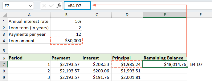

   
2. For the second and all subsequent periods, calculate the remaining balance by subtracting the current period's principal payment from the previous period's balance. Please apply the following formula into cell E8:

   =E7-D8

    Note: The reference to the balance cell should be relative, so it updates as you drag the formula down.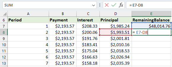
   
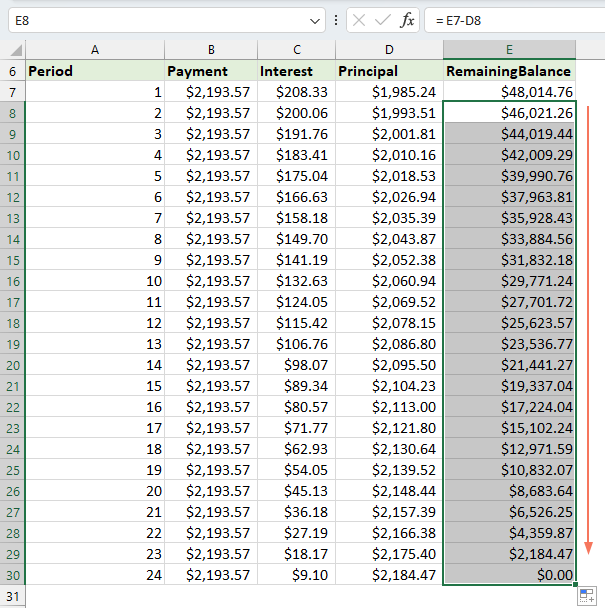
3. And then drag the fill handle down to the column. As you can see, each cell will automatically adjust to calculate the remaining balance based on the updated principal payments.
   

⭐️ Step 6: Make a loan summary

After setting up your detailed amortization schedule, creating a loan summary can provide a quick overview of the key aspects of your loan. This summary will typically include the total cost of the loan, the total interest paid.

● To calculate total payments:

=SUM(B7:B30)

● To calculate total interest:

=SUM(C7:C30)

⭐️ Result:

Now, a simple yet comprehensive loan amortization schedule has been successfully created. see screenshot:

Create an amortization schedule for a variable number of periods

In the previous example, we create a loan repayment schedule for a fixed number of payments. This approach is perfect for handling a specific loan or mortgage where the terms don't change.

But, if you're looking to create a flexible amortization schedule that can be repeatedly used for loans with varying periods, allowing you to modify the number of payments as required for different loan scenarios, you'll need to follow a more detailed method.

⭐️ Step 1: Set up the loan information and amortization table

1. Enter the relative loan information, such as annual interest rate, loan term in years, number of payments per year and loan amount into the cells as following screenshot shown:
   
2. Then, create an amortization table in Excel with the specified labels, such as Period, Payment, Interest, Principal, Remaining Balance in cells A7:E7.
3. In the Period column, input the highest number of payments you might consider for any loan, for example, fill the numbers ranging from 1 to 360. This can cover a standard 30-year loan if you're making monthly payments.
   

⭐️ Step 2: Modify the payment, interest and principle formulas with IF function

Enter the following formulas in the corresponding cells, and then drag the fill handle to extend these formulas down to the maximum number of payment periods you’ve set.

● Payment formula:

Normally, you use the PMT function to calculate payment. To incorporate an IF statement, the syntax formula is:

So the formulas is this:

=IF(A7<=$B$2*$B$3, -PMT($B$1/$B$3, $B$2*$B$3, $B$4), "")

● Interest formula:

The syntax formula is:

So the formulas is this:

=IF(A7<=$B$2*$B$3,-IPMT($B$1/$B$3, A7, $B$2*$B$3, $B$4), "")

● Principle formula:

The syntax formula is:

So the formulas is this:

=IF(A7<=$B$2*$B$3,-PPMT($B$1/$B$3, A7, $B$2*$B$3, $B$4), "")

⭐️ Step 3: Adjust the remaining balance formula

For the remaining balance, you might usually subtract the principal from the previous balance. With an IF statement, modify it as:

● The First balance cell:(E7)

=B4-D7

● The second balance cell:(E8)

=IF(A8<=$B$2*$B$3, E7-D8, "") 

⭐️ Step 4: Make a loan summary

After you've set up the amortization schedule with the modified formulas, the next step is to create a loan summary.

● To calculate total payments:

=SUM(B7:B366)

● To calculate total interest:

=SUM(C7:C366)

⭐️ Result:

Now, you have a comprehensive and dynamic amortization schedule in Excel, complete with a detailed loan summary. Whenever you adjust the payment period term, the entire amortization schedule will automatically update to reflect these changes. See the demo below:

Create an amortization schedule with extra payments

By making additional payments beyond the scheduled ones, a loan can be paid off more quickly. An amortization schedule that incorporates extra payments, when created in Excel, demonstrates how these additional payments can hasten the loan's payoff and decrease the total interest paid. Here's how you can set it up:

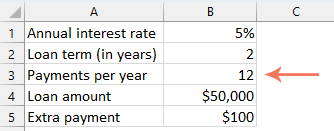
⭐️ Step 1: Set up the loan information and amortization table

1. Enter the relative loan information, such as annual interest rate, loan term in years, number of payments per year, loan amount and extra payment into the cells as following screenshot shown:
   
2. Then, calculate the scheduled payment.
   In addition to the input cells, another predefined cell is needed for our subsequent computations - the scheduled payment amount. This is the regular payment amount on a loan assuming no additional payments are made. Please apply the following formula into cell B6:

   =IFERROR(-PMT($B$1/$B$3, $B$2*$B$3, $B$4),"")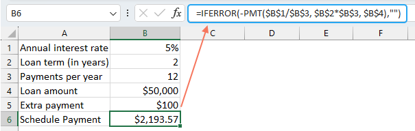

   
   
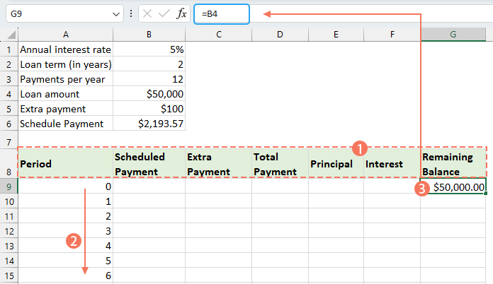
3. Then, create an amortization table in Excel:
   • Set the specified labels, such as Period, Schedule Payment, Extra Payment, Total Payment, Interest, Principal, Remaining Balance in cells A8:G8;
   • In the Period column, input the highest number of payments you might consider for any loan. For example, fill the numbers ranging from 0 to 360. This can cover a standard 30-year loan if you're making monthly payments;
   • For Period 0 (row 9 in our case), retrieve the Balance value with this formula =B4, which corresponds to the initial loan amount. All other cells in this row should be left blank.
   • 

⭐️ Step 2: Crete the formulas for amortization schedule with extra payments

Enter the following formulas in the corresponding cells one by one. To enhance error handling, we encase this and all future formulas within the IFERROR function. This approach helps avoid multiple potential errors that could arise if any of the input cells are left blank or hold incorrect values.

● Calculate the scheduled payment:

Enter the following formula into cell B10:

=IFERROR(IF($B$6<=G9, $B$6, G9+G9*$B$1/$B$3), "")

● Calculate the extra payment:

Enter the following formula into cell C10:

=IFERROR(IF($B$5<G9-E10,$B$5, G9-E10), "")

● Calculate the total payment:

Enter the following formula into cell D10:

=IFERROR(B10+C10, "")

● Calculate the principal:

Enter the following formula into cell E10:

=IFERROR(IF(B10>0, MIN(B10-F10, G9), 0), "")

● Calculate the interest:

Enter the following formula into cell F10:

=IFERROR(IF(B10>0, $B$1/$B$3*G9, 0), "")

● Calculate the remaining balance

Enter the following formula into cell G10:

=IFERROR(IF(G9 >0, G9-E10-C10, 0), "")

Once you have completed each of the formulas, select the cell range B10:G10, and use the fill handle to drag and extend these formulas down through the entire set of payment periods. For any periods not utilized, the cells will show 0s. See screenshot:

⭐️ Step 3: Make a loan summary

● Get scheduled number of payments:

=B2:B3

● Get actual number of payments:

=COUNTIF(D10:D369,">"&0)

● Get total extra payments:

=SUM(C10:C369)

● Get total interest:

=SUM(F10:F369)

⭐️ Result:

By following these steps, you create a dynamic amortization schedule in Excel that accounts for extra payments.

Create an amortization schedule by using Excel template

Creating an amortization schedule in Excel using a template is a straightforward and time-efficient method. Excel provides built-in templates that automatically calculate each payment's interest, principal, and remaining balance. Here's how to create an amortization schedule using an Excel template:

1. Click File > New, in the search box, type amortization schedule, and press Enter key. Then, select the template that best fits your needs by clicking on it. For example, here, I will select Simple loan calculator template. See screenshot:
   
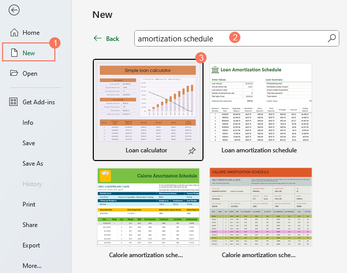
2. Once you've selected a template, click on the Create button to open it as a new workbook.
3. Then, enter your own loan details, the template should automatically calculate and populate the schedule based on your inputs.
4. At last, save your new amortization schedule workbook.