Create a hyperlink to another worksheet in the same workbook
Microsoft Excel is a versatile powerhouse for data organization and analysis, and one of its most valuable features is the ability to create hyperlinks. Hyperlinks enable you to effortlessly navigate between various worksheets within the same workbook, enhancing accessibility and user-friendliness. In this comprehensive guide, we'll delve into creating, editing, and removing hyperlinks in Excel, with a primary focus on interconnecting worksheets within the same workbook.

Create a Hyperlink to another sheet in Excel
Creating hyperlinks to link other sheets in Excel is a valuable skill for seamless navigation between different worksheets in the same workbook. Here are four methods to create a hyperlink in Excel.
Create a hyperlink to another sheet by using the Hyperlink command
You can create a hyperlink to another worksheet in the same workbook by employing Excel's built-in "Hyperlink command". Here's how to do it:
Step 1: Select a cell in a sheet that you want to create a hyperlink to another sheet
Here I selected cell "A3" in the "Index" sheet.

Step 2: Navigate to the Insert tab and click Link

Step 3: In the Insert Hyperlink dialog box, please do as follows:
1. Click the "Place in This Document" button in the left "Link to" box.
2. Click on the desired worksheet in the "Or select a place in this document" box to set it as the destination for your hyperlink; here I selected the "Sales" sheet.
3. Enter the cell address in the "Type the cell reference" box if you want to hyperlink to a specific cell in the chosen sheet Sales; Here I entered cell "D1".
4. Enter the text you want to display for the hyperlink in the "Text to display "box; Here I input "Sales".

5. Click "OK".
Result
Now cell "A3" in the "Index" sheet has a hyperlink to the specified cell "D1" in the "Sales" sheet within the same workbook. You can hover over the hyperlink and click on it to go to the specified cell D1 in Sales sheet.

Quickly create hyperlinks to each worksheet in one sheet with Kutools
To create individual hyperlinks to each worksheet within the same workbook, the conventional approach requires the repetitive creation of separate hyperlinks for each worksheet, a time-consuming and labor-intensive task. However, with "Kutools for Excel"'s "Create List of Sheet Names "utility, you can quickly create a hyperlink for each worksheet in one worksheet, significantly reducing manual effort and streamlining the process.
After downloading and installing Kutools for Excel, select "Kutools Plus "> "Worksheet " > "Create List of Sheet Names". In the "Create List of Sheet Names" dialog box, please do as follows.
- In the "Sheet Index Styles" section, check the "Contains a list of hyperlinks "option; (Here, you can also create buttons to link to other sheets as you need.)
- In the "Specify sheet name for Sheet Index" box, type a name for the new worksheet where will the hyperlinks will be located;
- In the "Insert the Sheet Index in" drop-down list, specify the position for the new Index sheet;
- Click "OK".

Result
Now hyperlinks to each worksheet are inserted in the newly-created "Index" sheet. You can click on any of the hyperlinks to quickly navigate to other worksheets.

Create a hyperlink to another sheet by using the HYPERLINK Function
With the "HYPERLINK" function, you also can create a hyperlink to another sheet within the same workbook. Clicking on the cell with the "HYPERLINK function" will take you to the specified sheet.
Step 1: Click on the cell where you want to create the hyperlink
Here I selected cell "A3" in the "Index" sheet.

Step 2: Enter the HYPERLINK formula
Type the "HYPERLINK "formula below and press "Enter" key.
=HYPERLINK("#Sales!D1", "Sales data")- "#Sales!D1": The destination of the hyperlink. In this case, it is a reference to a specific cell (cell "D1") within the sheet named "Sales".
- "Sales data": The text that will be displayed for the hyperlink. In this formula, it will appear as the clickable link text "Sales data".
Result
Now the formula creates a hyperlink with the text "Sales data" in cell "A3" of the "Index" sheet. When you click on it, it will take you to cell "D1" in the "Sales" sheet within the same workbook.

Create a hyperlink to another sheet by using the Drag-and-Drop Method
Excel's "drag-and-drop" feature provides a quick way to establish hyperlinks within the same workbook. To illustrate the process, we have provided a step-by-step "GIF" below.

Step-by-Step Descriptions:
1. Select the hyperlink destination cell in a sheet. Here I selected cell "D1" in the "Sales" sheet.

2. Point to one of the cell borders and press the "right mouse" button and hold it.
3. Press the "Alt" key, and drag the cell onto the other sheet’s tab. Here I selected the "Index" sheet.
4. Once the other sheet is activated, release the "Alt" key, and keep dragging the cell to the place where you want to insert a hyperlink. Here I selected cell "A3" in the "Index" sheet to insert the hyperlink.
5. Release the "right mouse" button. In the popping-up menu, click "Create Hyperlink Here".

Result
Now a hyperlink will appear in cell "A3" in the "Index "sheet, with the text from cell" D1" in the "Sales" sheet. When you click on it, it will take you to cell D1 in the Sales sheet within the same workbook.
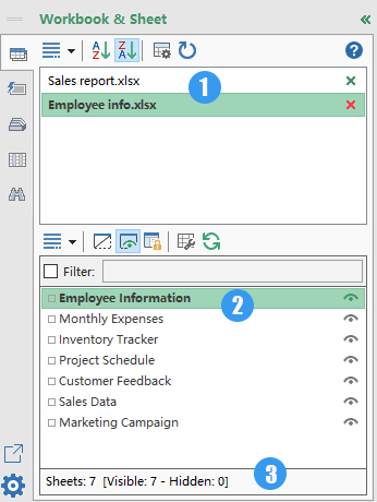
Navigation Pane:
List hyperlinks to each sheet
One click to effortlessly navigate through your Excel workbooks and worksheets using the Navigation Pane feature of Kutools for Excel.
- 📘 List all opening workbooks
- 📄 List all sheets of the active workbook
- 📊 Show the total number of sheets
🚀 Kutools for Excel: Your Time-Saving Excel Companion
Edit a Hyperlink in Excel
After creating a hyperlink, you may need to modify it to change the link destination, link text or adjust its format. In this section, we will show you two methods to edit a hyperlink.
Change the link destination/link text
To modify the destination or text of an existing hyperlink, please do as follows:
Step 1: Right-click on the hyperlink and select Edit Hyperlink from the drop-down menu

Step 2: In the popping-up Edit Hyperlink dialog, please do as follows:
You can make the desired changes to the "link text" or "link location" or both. For example, I want to change the link destination to "C1" in the "Expenses" sheet, and change the link text to "Expenses".
1. Click on the "Expenses" sheet in the "Or select a place in this document" box.
2. Enter cell" C1 "in the "Type the cell reference" box.
3. Enter the text "Expenses" in the "Text to display" box.

4. Click "OK".
Result
Now the link destination and link text are modified successfully.

Modify the hyperlink format
Excel hyperlinks are initially displayed with a traditional underlined blue formatting by default. To modify the default format of a hyperlink, follow these steps:
Step 1: Click on the cell containing the hyperlink.
Step 2: Navigate to the Home tab and locate the Styles group.
- Right-click on "Hyperlink" and select "Modify" to change the format of hyperlinks that have not been clicked.
- Or right-click on "Followed Hyperlink" and select "Modify" to adjust the formatting of hyperlinks that have been clicked.

Step 3: In the popping-up "Style" dialog box, click Format.

Step 4: In the Format Cells dialog, modify the hyperlink alignment, font, and fill color as you need
Go to the "Alignment"tab, or the "Font" tab, or the "Fill" tab to make necessary changes. Here I changed the font of the hyperlink under the "Font" tab. Click "OK" to save the changes.

Result
Now the format of the hyperlink has been changed successfully.

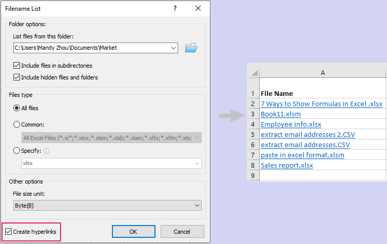
🌟 Create multiple hyperlinks to all workbooks/files in one folder 🌟
Kutools for Excel’s Filename List utility can batch add multiple hyperlinks to all files or one type of files in a certain folder, such as create hyperlinks to all workbooks, all word documents, or all text files, etc. Say goodbye to file chaos and hello to streamlined organization! 💪
📊 Kutools for Excel: Your Time-Saving Excel Companion 🚀
Download NowRemove a Hyperlink in Excel
Sometimes, you might want to remove hyperlinks without losing the formatting or content associated with it. In this section, we will explore two methods to help you achieve this goal.
Remove a hyperlink by using the Remove Hyperlink feature
Excel provides a straightforward way to remove a hyperlink using the "Remove Hyperlink" feature. Simply "right-click" on the cell containing the hyperlink and select "Remove Hyperlink" from the drop-down menu.

Now the hyperlink is removed while the link text is kept in the cell.

- If you want to delete a hyperlink and the link text that represents it, you should right-click the cell that contains the hyperlink and select "Clear Contents" from the drop-down menu.
- To remove hyperlinks from multiple cells, select the cells that contain hyperlinks and right-click on any cell of the selected cells and select "Remove hyperlinks" from the drop-down menu.
Easily remove hyperlinks without losing formatting using a smart tool
If you use the Remove Hyperlink feature to remove a hyperlink in Excel, the formatting of the hyperlink will be cleared. But we sometimes do need to keep the formatting, such as background color, font, size. Don’t worry. The "Remove Hyperlinks Without Losing Formatting" feature of "Kutools for Excel" can remove the hyperlinks while keeping the formatting, no matter in "a selected range", "an active sheet", "multiple selected sheets", or "the entire workbook". In this case, we need to remove hyperlinks in selected cells while keeping the formatting.
After downloading and installing Kutools for Excel, firstly select cells where you want to delete the hyperlinks, then click "Kutools" > "Link" > "Remove Hyperlinks Without Losing Formatting". Select "In selected Range" from the drop-down menu.

Now all hyperlinks in selected cells are removed at once but the formatting is retained as needed.

Related articles
How to insert bullet points in text box or specify cells in Excel?
This tutorial is talking about how to insert bullet points in a text box or multiple cells in Excel.
How to insert/apply bullets and numbering into multiple cells in Excel?
Apart from copying the bullets and numbering from Word documents to workbook, the following tricky ways will help you apply the bullets and numbering in cells of Excel quickly.
How to quickly insert multiple checkboxes in Excel?
How can we quickly insert multiple check boxes in Excel? Please follow these tricky methods in Excel:
How to add check mark in a cell with double clicking in Excel?
This article will show you a VBA method to easily add check mark in a cell with double clicking only.
Best Office Productivity Tools
Supercharge Your Excel Skills with Kutools for Excel, and Experience Efficiency Like Never Before. Kutools for Excel Offers Over 300 Advanced Features to Boost Productivity and Save Time. Click Here to Get The Feature You Need The Most...
Office Tab Brings Tabbed interface to Office, and Make Your Work Much Easier
- Enable tabbed editing and reading in Word, Excel, PowerPoint, Publisher, Access, Visio and Project.
- Open and create multiple documents in new tabs of the same window, rather than in new windows.
- Increases your productivity by 50%, and reduces hundreds of mouse clicks for you every day!
Table of contents
- Video: Create a hyperlink in Excel
- Create a hyperlink to another sheet in Excel
- By using the Hyperlink command
- Quickly create hyperlinks to each worksheet in one sheet with Kutools
- By using the HYPERLINK function
- By using the drag-and-drop method
- Edit a hyperlink in Excel
- Change the link destination/link text
- Modify the hyperlink format
- Remove a hyperlink in Excel
- By using the Remove Hyperlink feature
- Easily remove hyperlinks without losing formatting using a smart tool
- Related articles
- The Best Office Productivity Tools
- Comments