Excel DB Function

If you want to follow along with this tutorial, please download the example spreadsheet.

Description

The DB function returns the depreciation of an asset for a specified period by using a fixed-declining balance method.

Syntax and arguments

Formula syntax

Arguments

Return Value

The DB function returns a numeric value in currency format.

Errors

1. If the arguments are non-numeric value, the function returns #VALUE! error value.

2. If anyone of below occurs, the function returns ##NUM! error value:

• Cost < 0, or salvage < 0;
• Life or period <= 0;
• Month <=0, or month > 12;
• Period > life;

Remarks

1. Both of the life and period must be in the same unit. For instance, the life is calculated in yearly, the period must be calculated in yearly too.

2. The fixed-declining balance method computes the depreciation of asset at a fixed rate. The formula used in DB function to calculate the depreciation for a period is:

=(Cost – Total depreciation from prior periods) * Rate

Where

Rate = 1 – ((salvage / cost) ^ (1 / life)).

However, different formulas are used for first and last period (first year, and the end of the depreciation).

For the first period, DB function uses the below formula:

=Cost * Rate * Month / 12

For the last period, DB function uses the below formula:

=((Cost – Total depreciation from prior periods) * Rate * (12 – month)) / 12

Version

Excel 2003 or later

Usage and Examples

Example 1 when argument month is omitted

Supposing the cost, salvage, life and periods (1-5) are listed in the table B3:G8 and months are omitted, to calculate the depreciation of the asset in each period, please use below formula:

=DB(C3,C4,C5,C6)

Press Enter key to get the depreciation of first period.

Then select first result, drag autofill handle over the cells to calculate the depreciations in other periods.

Example 2 when argument month is less than 12

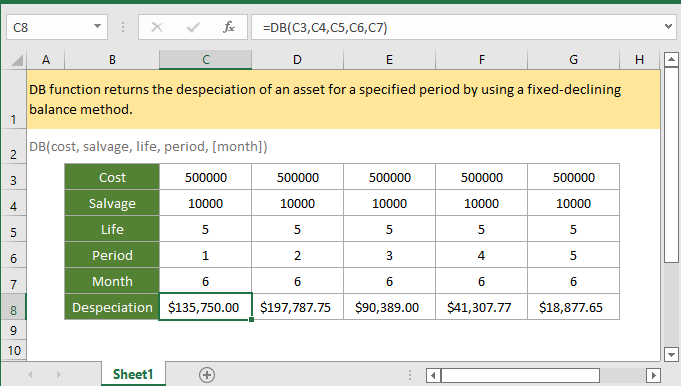
Supposing in the table B3:G8 which lists the cost, salvage, life and periods (1-5), and the month is 6, to calculate the depreciation of the asset in each period, please use below formula:

=DB(C3,C4,C5,C6,C7)

Press Enter key to get the depreciation of first period.

Then select first result, drag autofill handle over the cells to calculate the depreciations in other periods.

In this case, in the first year, DB only depreciates over 6 months, and in the second year, DB depreciates over 18 months (6 months in year 1, and 12 months in year 2).

Relative Functions:

• Excel CUMIPMT Function
  The CUMIPMT function returns the cumulative interest paid on a load between the start period and end period.

• Excel ACCRINT Function
  The ACCRINT function returns the accrued interest on periodic interest-paying securities.

• Excel ACCRINTM Function
  The ACCRINTM function returns the accrued interest for a security that pays interest at maturity.

• Excel AMORDEGRC Function
  The AMORDEGRC function returns the linear depreciation of an asset for each accounting period by applying a depreciation coefficient based on the lifetime of the assets.