Excel GETPIVOTDATA function

- Example1: Basic usage of the GETPIVOTDATA function
- Example2: How to avoid error values if the argument is date or time in GETPIVOTDATA function
Description
The GETPIVOTDATA function queries a pivot table and returns data based on the pivot table structure.
Syntax and arguments
Formula syntax
| =GETPIVOTDATA (data_field, pivot_table, [field1, item1], ...) |
Arguments
|
Return Value
The GETPIVOTDATA function returns data stored in the given pivot table.
Remarks
1) The calculated fields and custom calculation filed such as Grand Total and Sum of EachProwduct also can be as arguments in GETPIVOTDATA function.
2) If an item contains a date or time, the returned value may lose if the workbook is moved to another location and displayed as error value #REF!. For avoid this case, you can express date or time as series number such as show 12/3/2018 as 43437.
3) If argument pivot_table is not a cell or range in which a PivotTable is found, GETPIVOTDATA returns #REF!.
4) If the arguments are not visible in the given pivot table, the GETPIVOTDATA function returns the #REF! error value.
Usage and Examples
Example1: Basic usage of the GETPIVOTDATA function
1) Only first two required arguments:
=GETPIVOTDATA("StoreNorth",$A$3)
Explain:
If there are only two arguments in the GETPIVOTDARA function, it automatically returns the values in Grand Total field based on the given items name. In my example, it returns the Grand Total number of StoreNorth field in pivotable which is placed in Range A3:E9 (begins at Cell A3).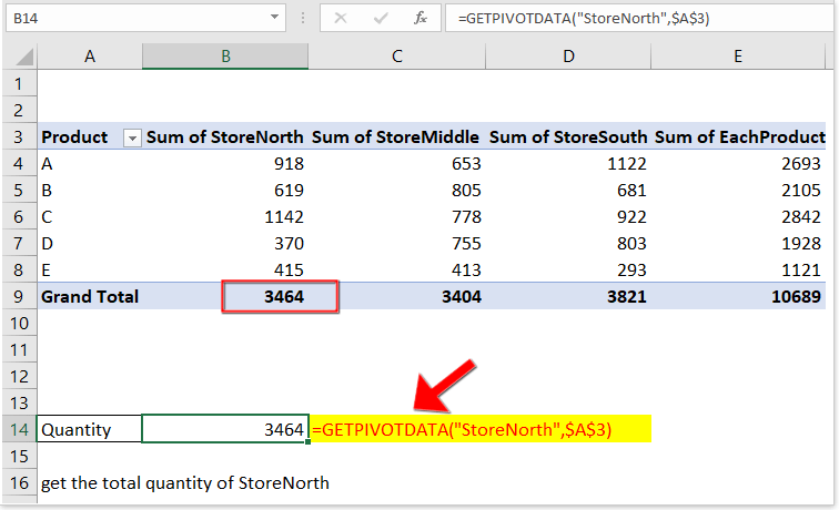
2) With data_field, pivot_table, field1, item1 argument
=GETPIVOTDATA("StoreNorth",$A$3,"Product","B")
Explain:
SouthNorth: data_field, the filed you want to retrieve value from;
A3: pivot_table, the first cell of the pivot table is Cell A3;
Product, B: filed_name, item_name, a pair which describes which value you want to return.
Example2: How to avoid error values if the argument is date or time in GETPIVOTDATA function
If the arguments in the GETPIVOTDATA function contain dates or time, the result may be changed to error value #REF! while the workbook is open in another destination as below screenshot shown: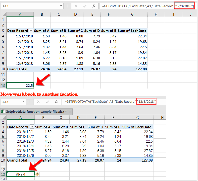
In this case, you can
1) Use the DATEVALUE function
=GETPIVOTDATA("EachDate",A3,"Date Record",DATEVALUE("12/3/2018"))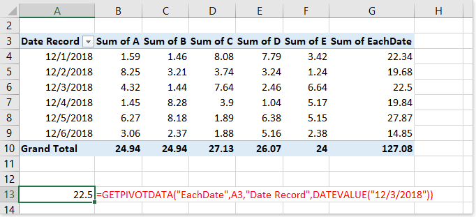
2) Use the DATE function
=GETPIVOTDATA("EachDate",A3,"Date Record",DATE(2018,12,3))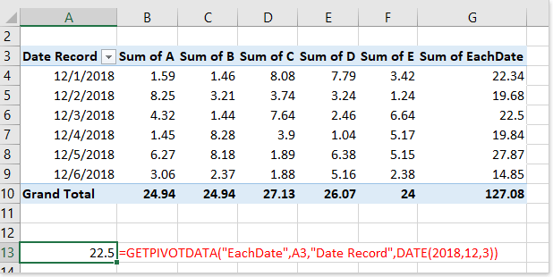
3) Refer to a cell with date
=GETPIVOTDATA("EachDate",A3,"Date Record",A12)
Sample File
The Best Office Productivity Tools
Kutools for Excel - Helps You To Stand Out From Crowd
Kutools for Excel Boasts Over 300 Features, Ensuring That What You Need is Just A Click Away...
Office Tab - Enable Tabbed Reading and Editing in Microsoft Office (include Excel)
- One second to switch between dozens of open documents!
- Reduce hundreds of mouse clicks for you every day, say goodbye to mouse hand.
- Increases your productivity by 50% when viewing and editing multiple documents.
- Brings Efficient Tabs to Office (include Excel), Just Like Chrome, Edge and Firefox.