Excel LOOKUP function
The Microsoft Excel LOOKUP function finds certain value in a one column or one row range, and return the corresponding value from another (one row or one column) range.
Tips: To lookup values, it is more recommended to use the VLOOKUP/HLOOKUP function and the new XLOOKUP function, because the LOOKUP function has more limitations in the calculation. Use the VLOOKUP/HLOOKUP function or the XLOOKUP function, depending on the Excel version you are using.
- VLOOKUP function: It performs a vertical lookup. Find things in a table or a range by row. It is available in Excel 2007 to 2021, and Excel for Microsoft 365.
- HLOOKUP function: It performs a horizontal lookup. Find things in the top row of a table or an array of values by column. It is available in Excel 2007 to 2021, and Excel for Microsoft 365.
- XLOOKUP function: The XLOOKUP function is the new lookup function that solves a lot of the issues that VLOOKUP and HLOOKUP had. It finds things in a table or a range in any direction (up, down, left, right), which is more easier to use and works faster than other lookup functions. It is only available in Excel for Microsoft 365.
Syntax
=LOOKUP (lookup_value, lookup_vector, [result_vector])
Arguments
Lookup_value (required): The value you will search for. It can be a number, a text or a reference to a cell containing the search value.
Lookup_vector (required): A single row or single column range to be searched. The value in this argument can be numbers, text or logical values.
Note: Values in this range must be sorted in ascending order, otherwise, LOOKUP might not return the correct value..
result_vector (optional): The LOOKUP function searches for the value in the look_up vector, and returns the result from the same column or row position in the result_vector. It is a one-row or one-column data which has the same size with the lookup_vector.
Return value
The LOOKUP function will return a value in a one column range.
Function Notes:
1. If the lookup number is smaller than all values in the lookup range, it will return a #N/A error value.
2. LOOKUP works based on approximate match, if the lookup value can’t be found exactly, it will match the next smallest value.
3. If there are multiple matched look_up values, it will match the last value.
4. The LOOKUP function is not case-sensitive.
Examples
Example 1: Use LOOKUP function to find a value with one criterion
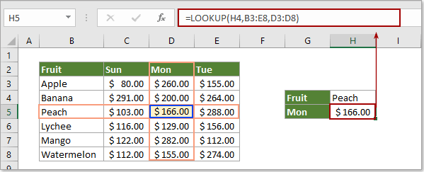
As the below screenshot shown, you need to find Peach in the table range, and return the corresponding result in the Mon column, you can achieve it as follows.
Select a blank cell, copy the below formula into it and press the Enter key.
=LOOKUP(H4,B3:E8,D3:D8)
Notes:
- H4 is the reference cell containing the search value “Peach”; B3:E8 is the lookup range containing the search value and the result value; D3:D8 is the result value range.
- You can replace the H4 with "Peach" or B5 directly as you need.
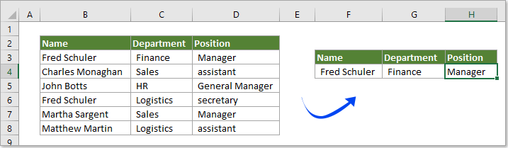
Example 2: LOOKUP function search for a value with multiple criteria
As below screenshot shown, there are duplicate names in different departments. For finding the position of a specific person (says Fred Schuler), you need to match the Name and Department criteria at the same time. Please do as follows.
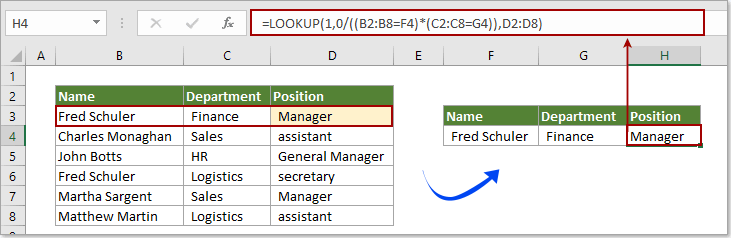
1. Select blank cell to place the result, copy the below formula into it and press the Enter key.
=LOOKUP(1,0/((B2:B8=F4)*(C2:C8=G4)),D2:D8)
Notes:
- In the formula, B2:B8 and C2:C8 are the column ranges containing the first and second look up values; F4 and G4 are the references to the cells containing the two criteria; D2:D8 is the result value range. Please change them based on your table range.
- This formula can also help.
=LOOKUP(1,0/((B2:B8&C2:C8=F4&G4)),D2:D8)
More Examples
How to vlookup and return matching data between two values in Excel?
The Best Office Productivity Tools
Kutools for Excel - Helps You To Stand Out From Crowd
Kutools for Excel Boasts Over 300 Features, Ensuring That What You Need is Just A Click Away...
Office Tab - Enable Tabbed Reading and Editing in Microsoft Office (include Excel)
- One second to switch between dozens of open documents!
- Reduce hundreds of mouse clicks for you every day, say goodbye to mouse hand.
- Increases your productivity by 50% when viewing and editing multiple documents.
- Brings Efficient Tabs to Office (include Excel), Just Like Chrome, Edge and Firefox.