Excel TEXTSPLIT function

The TEXTSPLIT function splits text strings by a given delimiter to an array across columns and rows.

Note: This function is only available in Excel for Microsoft 365 on the Insider channel.

Syntax

=TEXTSPLIT(text, col_delimiter, [row_delimiter], [ignore_empty], [match_mode], [pad_with])

Arguments

Remarks

Return value

It returns the split text string.

Example

Here we take some examples to demonstrate how to use the TEXTSPLIT function to split text under different conditions.

#Example 1: Split text by a delimiter into columns or rows

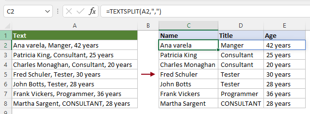
As shown in the screenshot below, to split the text in the cell A2 into columns or rows by comma, you can apply the TEXTSPLIT function as follows.

Split text horizontally into columns by commas

Select a cell, enter the following formula and press the Enter key.

The results are populated with split texts at the same time without using the AutoFill Handle.

=TEXTSPLIT(A2,",")

Split text vertically into rows by commas

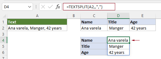
To split text vertically into rows by a given delimiter, you need to leave the col_delimiter argument blank and specify a delimiter for the row_delimiter argument. Please do as follows.

Select a cell, enter the following formula and press the Enter key.

The result cells are populated with split texts at the same time without using the AutoFill Handle.

=TEXTSPLIT(A2,,",")

#Example 2: Ignore empty cells when splitting text with the TEXTSPLIT function

As shown in the screenshot below, if the text string contains two or more consecutive delimiters without a value between them, by default, the TEXTSPLIT function will preserve empty cells when splitting text. To ignore empty cells when splitting, you can apply the TEXTSPLIT function as follows.

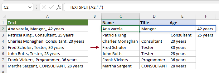
Select a blank cell, enter the following formula and press Enter to get all split texts and ignore the empty cells. If there is a list of texts to split, please select the result cell and drag its AutoFill Handle down to get the rest of the results.

=TEXTSPLIT(A2,",",,TRUE)

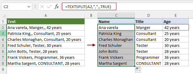
Note: In this formula, the logical value “TRUE” is provided as the ignore_empty argument.

#Example 3: Split text case-sensitive or case-insensitive

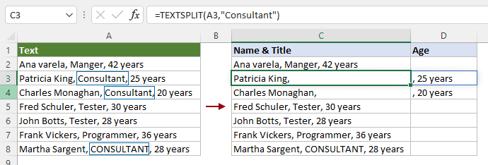
By default, the TEXTSPLIT function is case sensitive as the match_mode is set to 0 or left blank.

As shown in the screenshot below, the match_mode argument in the TEXTSPLIT function is left blank, so it only searches for an exact match of the text “Consultant” in the specified text string.

=TEXTSPLIT(A2,"Consultant")

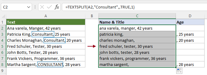
If you don’t want to make exact match search, for example, you need to search for the text that includes both “Consultant” and “CONSULTANT”, in this case, you can specify the match_mode argument as 1 to get it done.

Select a blank cell, enter the formula below and press the Enter key. Select this result cell and drag its AutoFill Handle down to get the rest of the results.

=TEXTSPLIT(A2,"Consultant",,TRUE,1)

#Example 4: Split text into rows and columns at the same time

To split text into rows and columns as the same time by using the TEXTSPLIT function, you need to specify both the col_delimiter and the row_delimiter arguments in the formula at the same time.

As shown in the table below, you can enter the following formula into cell C2 and press the Enter key to get the split texts in corresponding rows and columns at the same time.

=TEXTSPLIT(A2,":", ",")

Note: In this case, a colon “:” is provided as the col_delimiter argument and a comma “,” is provided as the row_delimiter argument.

#Example 4: Customize a value to pad missing values in 2D array

When using the TEXTSPLIT function to split text into both rows and columns at the same time, Excel returns #N/A errors in the result if there are missing values in the original text string.

As shown in the screenshot below, since there is no colon “:” after the text Released date, Excel returns #N/A next to “Released date”.

If you need to pad all missing values with a dash (-) character in the 2D array instead of #N/A error, you just need to specify the last argument “pad_with” as “-” to get it done.

Select a blank cell, enter the following formula and press the Enter key to get all split texts in rows and columns.

=TEXTSPLIT(A2,":",",",,,"-")

#Example 5: Split text by multiple delimiters

The TEXTSPLIT function allows multiple delimiters to be used to split text at the same time. However, the delimiters must be enclosed in an array constant and separated by commas, such as {“delimiter1”,”delimiter2”,...}.

The text string in the table below contains two delimiters “-” and “,”, to split the text by these two delimiters, you need to apply the TEXTSPLIT function as follows.

Select a blank cell, enter the following formula and press the Enter key.

=TEXTSPLIT(A2,{"-",","})

Note: In this formula, the col_delimiter argument is specified as {"-",","}.

Related Functions