Greetings,
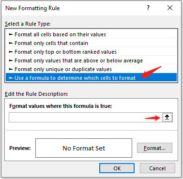
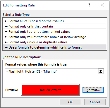
I am creating an assignment log for my work and I have Sheet1 acting as a display of who has what equipment assigned to them. This info is updated from other sheets. On these other sheets, I have a conditional formatting drop down list with 5 colors essentially White, Red, Yellow, Green and Cyan for Not Issued, Missing, Out of Service, Issued and Returned respectively.
I have the item that is issued with an ID number such as FL-01 to indicate which item they were issued. I would like to retain that information in its cell but be updated with the corresponding color when I select it from the drop down list.
For confidentiality reasons, I am unable to upload the file but I can say that I have 9 columns from C to L and 29 rows. Each column C through L has its own sheet that corresponds to it.
Another example: I want Column D with FL-01 in Cell D8 to show Green from the Drop Down Cell in C-8 on Sheet2 and change when I change the Drop Down option.
Thanks in advance,
Viepyr

