Hi there,

Currently we don't have such a feature to directly do that for you. However, there is a workaround with Kutools' features (you can download and try it for free for 30 days):

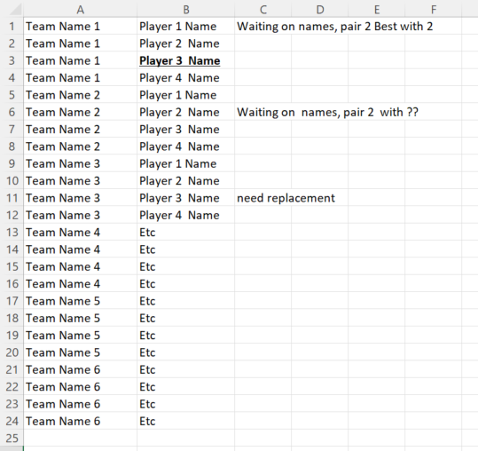
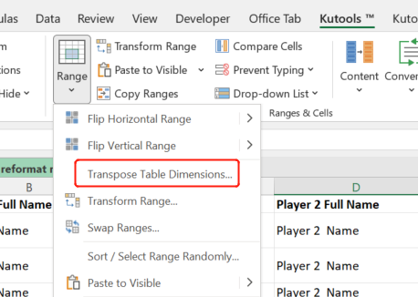
1. Select the range 'How data currently exports'!$A$1:$I$7, then on the Kutools tab, click Range > Transpose Table Dimensions.



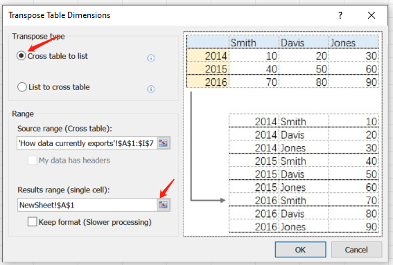
2. In the pop-up dialog, choose Cross table to list, and click the range-selection icon under the Results range section to select a cell where you want to output the result (here I created a new sheet and select the cell A1).



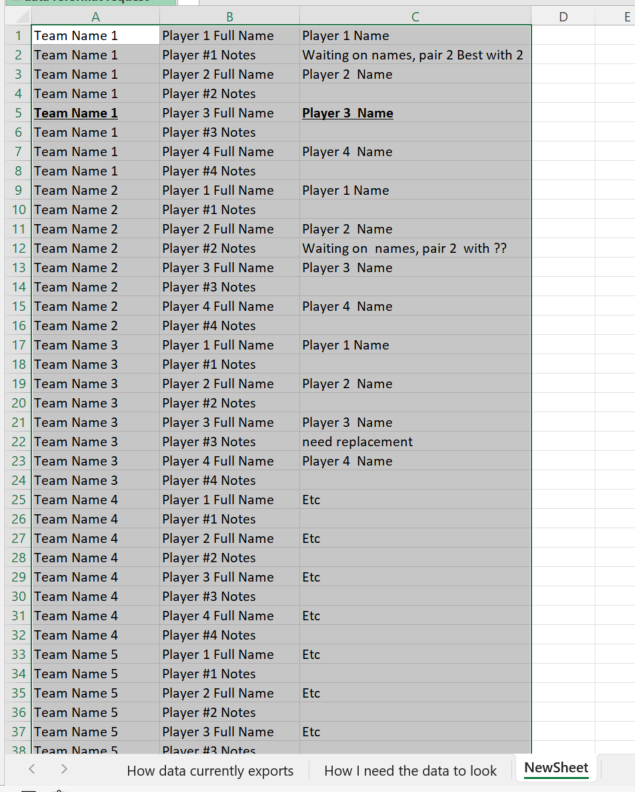
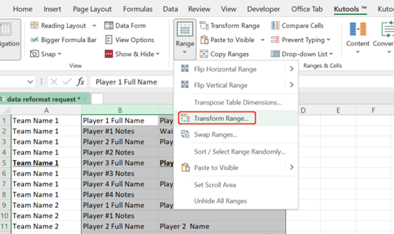
3. You will see the result as shown below. Now select the range C1:C48 and then on the Kutools tab, click Range > Transform Range.




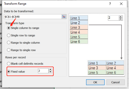
4. In the pop-up dialog, choose Single column to range. In the Fixed value box, enter 2. Once finished, click OK.



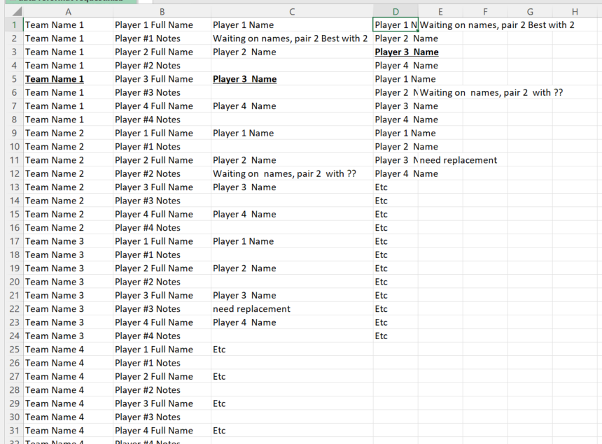
5. Specify the output range in the next pop-up dialog (here I select D1). You will see the results as shown below.



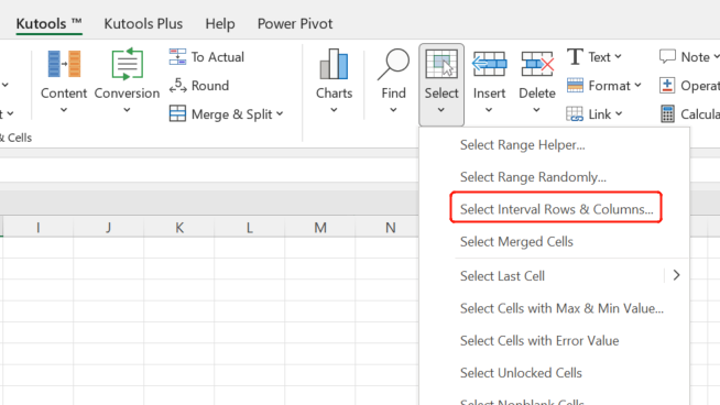
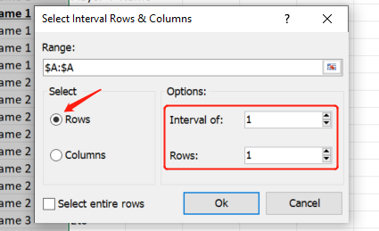
6. Delete the column B and C. Select column A and then click Select > Select Interval Rows and Columns.



7. In the pop-up dialog, choose Rows. Under Options, set 1 for both interval and rows number. Once finished, click OK. (Do not check Select entire rows)



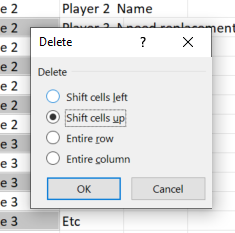
8. Right-click on any of the selected cells, and then click Delete. In the pop-up dialog, select Shift cells up.



9. Now you will see the result as shown below. You can add headers for the table.