Highlight every other row or column in Excel - Step by step guide

In a large worksheet, highlighting or filling every other or every nth row or column improves data visibility and readability. It not only makes the worksheet look neater but also helps you understand the data faster. In this article, we'll guide you through various methods to shade every other or nth row or column, helping you present your data in a more appealing and straightforward manner.

Highlight every other row or column

• By applying Table style
• By using a quick feature - Kutools for Excel
• By using Conditional Formatting

Alternate row color based on value changes

• By using Conditional Formatting
• By using a powerful feature – Kutools for Excel

Video: Highlight every other row or column

 Highlight every other row or column  

In this section, we'll show you three simple ways to shade every other row or column in Excel. This will help make your data look better and be easier to read.

Highlight every other row or column by applying Table style

Table styles offer a convenient and swift tool to easily highlight every other row or column in your data. Please do with the following steps:

Step 1: Select the data range that you want to shade

Step 2: Apply the Table style

1. Click "Home" > "Format as Table", and then choose a table style that has alternate row shading, see screenshot:
   
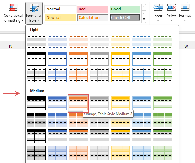
2. Then, in a prompt "Create Table" dialog bob, click "OK", see screenshot:
   Note: If there is no headers in the selected range, untick My table has headers checkbox.
   

Result:

Now, the selected data has been shaded alternately as shown in the following screenshot:

Highlight every other or nth row or column by using a quick feature - Kutools for Excel

Do you want to easily highlight every other or specific row/column in Excel? The "Alternate Row / Column Shading" feature of "Kutools for Excel" can make your data stand out and organized. No complicated steps required, in just a few simple clicks, make your spreadsheet look more professional and clearer!

Select the data range, and then click "Kutools" > "Format" > "Alternate Row / Column Shading" to enable this feature. In the "Alternate Row / Column Shading" dialog box, please do the following operations:

1. Select "Rows" or "Columns" you wish to shade from the "Apply shading to" section;
2. Choose "Conditional formatting or Standard formatting" from the "Shading method";
3. Specify a shade color for highlighting the rows from the "Shade color" drop down;
4. Specify the interval at which you want to shade rows from the "Shade every" scroll box, such as every other row, every third row, every fourth row, and so on;
5. At last, click "OK" button.
   

Result:

Shade every other row	Shade every other column

Highlight every other or nth row or column by using Conditional Formatting

In Excel, Conditional Formatting stands out as an invaluable feature, enabling users to dynamically alternate colors for rows or columns. In this section, we'll dive into some formula examples to help you alternate row colors in different ways:

• Shade every other or nth row / column
• Shade alternating groups of n rows / columns

Shade every other or nth row / column

To highlight every other or nth row or column, you can create a formula within the "Conditional Formatting", please follow these steps:

Step 1: Select the data range that you want to shade

Step 2: Apply the Conditional Formatting feature

1. Click "Home" > "Conditional Formatting" > "New Rule", see screenshot:
   
2. In the "New Formatting Rule" dialog box:
   • 2.1 Click "Use a formula to determine which cells to format" from the "Select a Rule Type" list box;
   • 2.2 Type any one of the below formulas into the "Format values where this formula is true" textbox you need:
     Shade every odd row:

     =MOD(ROW(),2)=1

     Shade every even row:

     =MOD(ROW(),2)=0

   • 2.3 Then, click "Format" button.
     
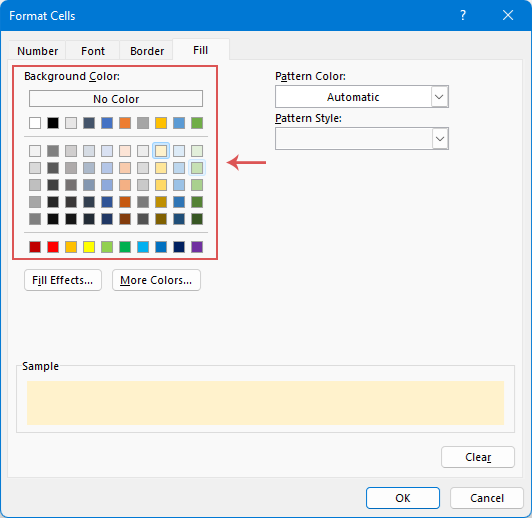
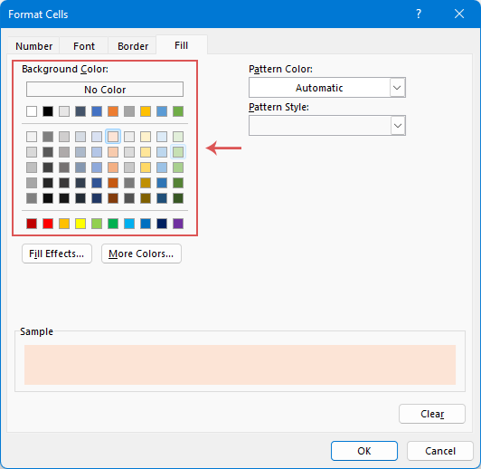
3. In the "Format Cells" dialog box, under the "Fill" tab, specify one color you want to fill the rows, and then, click "OK".
   
4. When it returns to the "New Formatting Rule" dialog box, click "OK".

Result:

Shade every odd row	Shade every even column

Shade alternating groups of n rows / columns

If you want to shade every n rows or columns in Excel as following screenshot shown, a combination of the ROW, CEILING, and ISEVEN or ISODD functions paired with conditional formatting is your go-to solution. Here, we'll walk you through a step-by-step process to easily highlight alternating groups of n rows or columns.

Step 1: Select the data range that you want to shade

Step 2: Apply the Conditional Formatting feature

1. Click "Home" > "Conditional Formatting" > "New Rule" to go to the "New Formatting Rule" dialog box, in the popped-out dialog box, please do the following operations:
   • 1.1 Click "Use a formula to determine which cells to format" from the "Select a Rule Type" list box;
   • 1.2 Type any one of the below formulas into the Format values where this formula is true textbox you need:
     Shade alternate n rows from the first group:

     =ISODD(CEILING(ROW(),3)/3)

     Shade alternate n rows from the second group:

     =ISEVEN(CEILING(ROW(),3)/3)

   • 1.3 Then, click "Format" button.
     Note: in the above formulas, the number 3 indicates the group of rows that you want to shade alternately. You can change it to any other number you need.
     
2. In the "Format Cells" dialog box, under the "Fill" tab, specify one color you want to fill the rows, and then, click "OK".
   
3. When it returns to the "New Formatting Rule" dialog box, click "OK".

Result:

Shade alternate 3 rows from the first group	Shade alternate 3 rows from the second group

=ISODD(CEILING(COLUMN(),3)/3)

=ISEVEN(CEILING(COLUMN(),3)/3)

Alternate row color based on value changes

Sometimes, you may need to change row colors based on different cell values to make the data visually easier to analyze. For instance, if you have a range of data and you want to highlight rows where values in a specific column (column B) change, doing so allows for quicker identification of where the data shifts. This article will discuss two practical methods to accomplish this task in Excel.

Alternate row color based on value changes with Conditional Formatting

In Excel, using Conditional Formatting with a logical formula is a useful way to highlight rows where values change. This ensures that every adjustment in value is clearly and distinctly marked.

Step 1: Select the data range that you want to shade (exclude the header row)
Note: When using the following formulas, the data range must have header row, otherwise, an error will occur.

Step 2: Apply the Conditional Formatting feature

1. Click "Home" > "Conditional Formatting" > "New Rule" to go to the "New Formatting Rule" dialog box, in the popped-out dialog box, please do the following operations:
   • 1.1 Click "Use a formula to determine which cells to format" from the "Select a Rule Type" list box;
   • 1.2 Type any one of the below formulas into the "Format values where this formula is true" textbox you need:
     Shade rows based on value changes from the first group:

     =ISODD(MOD(SUMPRODUCT(--($B$1:$B1<>$B$2:$B2)),2))

     Shade rows based on value changes from the second group:

     =ISEVEN(MOD(SUMPRODUCT(--($B$1:$B1<>$B$2:$B2)),2))

   • 1.3 Then, click "Format" button.
     Note: in the above formulas, B1 is the header row of the column that you want to shade rows based on, B2 is the first cell in your data range.
     
2. In the "Format Cells" dialog box, under the "Fill" tab, specify one color you want to fill the rows, and then, click "OK".
   
3. When it returns to the "New Formatting Rule" dialog box, click "OK".

Result:

Shade rows when value changes from the first group	Shade rows when value changes from the second group

Alternate row color based on value changes with a powerful feature-Kutools for Excel

If the previous method seems a bit tough, there’s an easier way! You can use "Kutools for Excel". Its "Distinguish Differences" feature makes coloring rows by group really easy and fast. Not only can you change the colors of rows when values change, but you can also add borders, page breaks, or blank rows as needed, making your Excel data more organized and easier to understand.

Click "Kutools" > "Format" > "Distinguish Differences" to enable this feature. In the "Distinguish differences by key column" dialog box, please do the following operations:

1. In the "Range" box, specify the selection that you want to shade color;
2. In the "Key column" box, select the column that you want to shade color based on;
3. In the "Options" section, check the "Fill Color" option, and specify one color;
4. In the "Scope" section, choose "Selection" from the drop down;
5. At last, click "OK".
   

Result:

Whether you choose to use table style or Kutoosl for Excel or Conditional Formatting, you can easily add highlighting effects to your Excel data. Based on your specific needs and preferences, choose the method that suits you best for the task. If you're interested in exploring more Excel tips and tricks, our website offers thousands of tutorials, please click here to access them. Thank you for reading, and we look forward to providing you with more helpful information in the future!

Related Articles: