Easily create a horizontal waterfall chart in Excel

Normally, you can create a vertical waterfall chart quickly in Excel. Here recommend the Horizontal Waterfall Chart utility of Kutools for Excel. With this feature, you can easily create a horizontal waterfall chart or a mini horizontal waterfall chart in Excel.

Create a horizontal waterfall chart

You can do as follows to create a horizontal waterfall chart in Excel.

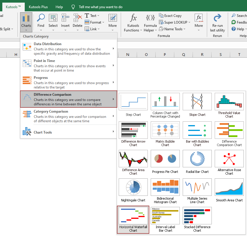
1. Click Kutools > Charts > Difference Comparison > Horizontal Waterfall Chart.

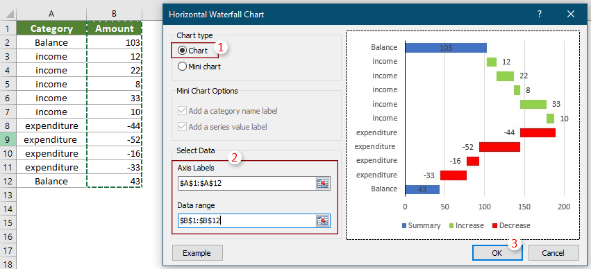
2. In the Horizontal Waterfall Chart dialog box, configure as follows.

2.1) In the Chart type section, choose the Chart option;

2.2) In the Select Data section:

Axis Labels: Select the axis labels data range;

Data range: Select the series data range.

2.3) Click OK.

3. A Kutools for Excel dialog box pops up, click Yes.

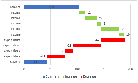
And then a horizontal waterfall chart is created as the below screenshot shown.

Create a mini horizontal waterfall chart

This feature can also help to create a mini horizontal waterfall chart in Excel cells. You can do as follows to get it done.

1. Click Kutools > Charts > Difference Comparison > Horizontal Waterfall Chart.

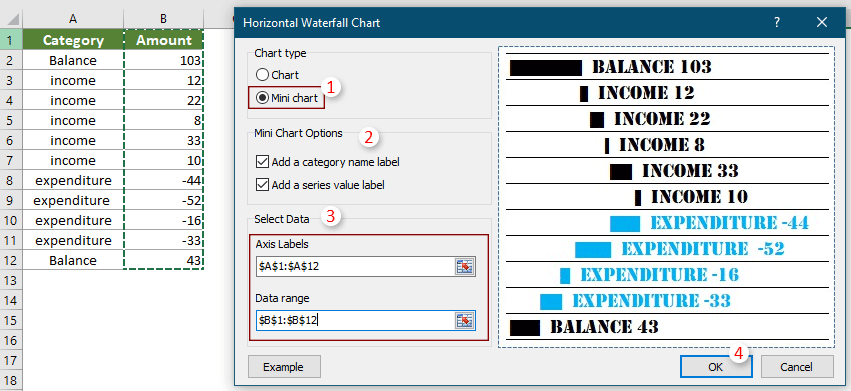
2. In the Horizontal Waterfall Chart dialog box, do the following settings.

2.1) In the Chart type section, choose the Mini chart option;

2.2) In the Mini Chart Options section, there are two options “Add a category name label” and “Add a series value label”, it’s optional to choose one of them, both of them, or none as you need;

2.3) In the Select Data section:

Axis Labels: Select the axis labels data range;

Data range: Select the series data range.

2.4) Click OK.

3. In the opening Kutools for Excel dialog box, click Yes.

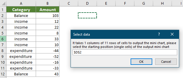
4. Then a Select data dialog box pops up, select a cell to output the mini chart, and then click OK.

Now a mini horizontal waterfall chart is created.

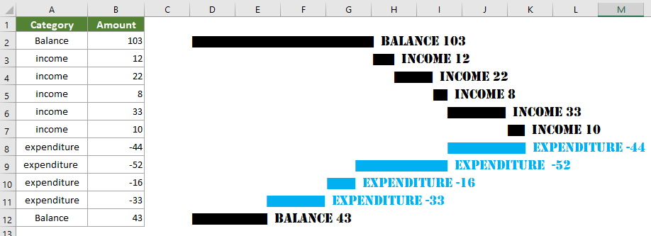
When choose both the “Add a category name label” and “Add a series value label” options in the Horizontal Waterfall Chart dialog box, you will get the mini chart as follows.

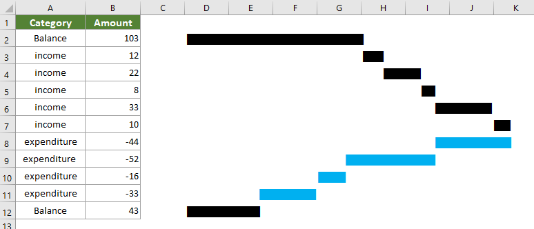
When none of them are chosen, you will get the mini chart as the below screenshot shown.

When choose one of them such as “Add a series value label”, you will get the result as follows.

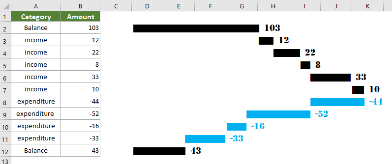
Notes:

  If you want to have a free trial ( 30-day) of this utility, please click to download it, and then go to apply the operation according above steps.

Kutools for Excel

The functionality described above is just one of 300 powerful functions of Kutools for Excel.

Designed for Excel(Office) 2019, 2016, 2013, 2010, 2007 and Office 365. Free download and use for 60 days.