How to easily compare cells by case sensitive or insensitive in Excel?
Supposing you have two lists with some duplicates in the same rows, and now you want to compare these two lists by case sensitive or insensitive as below screenshots shown, how can you quickly handle this task in Excel?


Compare cells case sensitive or insensitive with formulas
Compare two lists case sensitive or insensitive with Compare Range function
 Compare cells case sensitive or insensitive with formulas
In excel, to compare cells by case sensitive or insensitive, you can use formulas to solve.
1. Select a blank cell next to the compare cells, and type this formula =AND(EXACT(E1:E6,F1:F6)) into it, press Enter key, then drag the auto fill handle down to the cells. And False means the relative cells are not duplicate in case sensitive, and True means the cells are duplicate in case sensitive. See screenshots:

Tip:
1. To compare cells case insensitive, you can use this formula =AND(A1=B1), remember to press Shift + Ctrl + Enter keys to get the correct result.
2. In above formulas, E1:E6 and F1:F6 are the two lists of the cells.
| Never need to worry about long long formulas in Excel anymore! Kutools for Excel's Auto Text can add all formulas to a group as auto text, and liberate your brain! Know About Auto Text Get Free Trial |
||
Compare two lists case sensitive or insensitive with Compare Range function
But in sometimes, you may want to compare two lists case sensitive whose duplicates are not in the same rows as below screenshots shown, in this case, you can use Kutoolsfor Excel’s Select Same & Different Cells function.


| Kutools for Excel, with more than 300 handy functions, makes your jobs more easier. |
After free installing Kutools for Excel, please do as below:
1. Select the first list, and then click Kutools > Select > Select Same & Different Cells. See screenshot:

2. Then in the Compare Ranges dialog, following below operations. See screenshot:
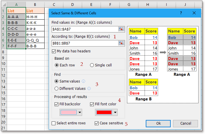
2) Check Each row from the Based on section; (if you do not want to compare the headers, check My data has headers option);
3) Check Same Values in the Find section, if you want to find the unique ones, check Different Values;
4) Specify the filled color and font color if you want to highlight the selected cells;
5) Check Case sensitive to compare two lists by case sensitive.
3. And click Ok, and a dialog pops out to remind you the number of selected cells.

4. Click OK to close dialogs. And you can see only the duplicates which match case sensitive are selected and highlighted.

Tip:If you uncheck Case sensitive in Compare Ranges dialog, you can see the comparing result:

Relative Articles:
- How to paste values to visible cells only in Excel?
- How to count and remove duplicates from a list in Excel?
- How to remove all duplicates but keep only one in Excel?
- How to count unique/duplicate dates in an Excel column?
Best Office Productivity Tools
Supercharge Your Excel Skills with Kutools for Excel, and Experience Efficiency Like Never Before. Kutools for Excel Offers Over 300 Advanced Features to Boost Productivity and Save Time. Click Here to Get The Feature You Need The Most...
")
Office Tab Brings Tabbed interface to Office, and Make Your Work Much Easier
- Enable tabbed editing and reading in Word, Excel, PowerPoint, Publisher, Access, Visio and Project.
- Open and create multiple documents in new tabs of the same window, rather than in new windows.
- Increases your productivity by 50%, and reduces hundreds of mouse clicks for you every day!
")