How to count number of peaks in a column of data in Excel?
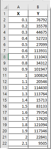
Supposing, two columns of data locates in your worksheet as the left screenshot shown, how to count the number of peaks in column B? Actually you can judge a cell value (such as B3) as a peak if it is simultaneously greater than B2 and B4. Otherwise, it is not a peak if it does not meet these two criteria. This article is talking about listing and counting all peaks in a column of data in Excel.
Count number of peaks in a column of data in Excel

The following formula can help you to count a number of peaks in a column of data directly in Excel.
1. Select a blank cell for placing the result, enter formula =SUMPRODUCT(--(B3:B17>B2:B16),--(B3:B17>B4:B18)) into the Formula Bar, then press the Enter key. See screenshot:

Note: In the formula, B3:B17 is the range from the third cell (including header cell) to the second last one of the list, B2:B16 is the range from the second cell (including header cell) to the antepenultimate one of the list, and finally B4:B18 is the range scope from the fourth cell (including header cell) to the last one of the list. Please change them as you need.
Mark all peaks in a scatter chart
Besides, you can easily figure out peaks of a column by creating a scatter chart and marking all peaks ion the chart. Please do as follows.
1. Select the cell - C3 which is adjacent to cell B3 (the second cell value of your list excluding the header), enter formula =IF(AND(B3>B2,B3>B4), "Peak","") into the Formula Bar and press the Enter key. Then drag the Fill Handle down to mark all peaks as below screenshot shown.

2. Select the column x and y, and click Insert > Insert Scatter (X, Y) or Bubble Chart > Scatter with Straight Lines and Markers to insert a scatter chart into the worksheet. See screenshot:

3. Press the Alt + F11 keys to open the Microsoft Visual Basic for Applications window.
4. In the Microsoft Visual Basic for Applications window, please click Insert > Module. Then copy and paste below VBA code into the Code window.
VBA code: Mark all peaks in a scatter chart
Sub CustomLabels()
    Dim xCount As Long, I As Long
    Dim xRg As Range, xCell As Range
    Dim xChar As ChartObject
    Dim xCharPoint As Point
    On Error Resume Next
    Set xRg = Range("C1")
    Set xChar = ActiveSheet.ChartObjects("Chart 1")
    If xChar Is Nothing Then Exit Sub
    xChar.Activate
    xCount = ActiveChart.SeriesCollection(1).Points.Count
    For I = 1 To xCount
        Set xCell = xRg(1).Offset(I, 0)
        If xCell.Value <> "" Then
            Set xCharPoint = ActiveChart.SeriesCollection(1).Points(I)
            xCharPoint.ApplyDataLabels
            xCharPoint.DataLabel.Text = xCell.Value
            xCharPoint.DataLabel.Left = xCharPoint.DataLabel.Left - 15
            xCharPoint.DataLabel.Top = xCharPoint.DataLabel.Top - 7
        End If
    Next
End SubNote: In the code, Chart 1 is the name of the created scatter chart, and “C1” is the first cell of the help column which contains the formula results you applied in step 1. Please change them based on your needs.
5. Press the F5 key to run the code. Then all peaks are marked on the scatter chart as below screenshot:

Best Office Productivity Tools
Supercharge Your Excel Skills with Kutools for Excel, and Experience Efficiency Like Never Before. Kutools for Excel Offers Over 300 Advanced Features to Boost Productivity and Save Time. Click Here to Get The Feature You Need The Most...
")
Office Tab Brings Tabbed interface to Office, and Make Your Work Much Easier
- Enable tabbed editing and reading in Word, Excel, PowerPoint, Publisher, Access, Visio and Project.
- Open and create multiple documents in new tabs of the same window, rather than in new windows.
- Increases your productivity by 50%, and reduces hundreds of mouse clicks for you every day!
")