Search and highlight specific data in Excel
When working with large datasets in Excel, it is often necessary not only to search for specific values but also to visually distinguish these values for data analysis, validation, or review purposes. Excel’s built-in Find and Replace feature can help you locate values; however, it doesn’t provide an automatic way to highlight the cells containing your search results. If you need to have the matching data stand out quickly—making subsequent editing, highlighting, or data checking more efficient—you may need additional methods to achieve this effect.
This guide introduces three practical ways to search for and highlight your results simultaneously in Excel. Each method has different advantages, suitable scenarios, and a few limitations you should be aware of before deciding which one to use. By understanding and applying these approaches, you can improve both the efficiency and accuracy of your data processing tasks.
➤ Highlight search results using VBA code
➤ Highlight search results using Conditional Formatting
➤ Highlight search results using a handy tool
➤ Highlight search results using Filter and manual coloring
➤ Highlight search results using an Excel helper column formula
If you wish to highlight all cells containing a particular value within an entire worksheet or a specific area, using a VBA macro offers a highly flexible solution in Excel. VBA can automate the searching and highlighting process, saving you time—especially when you’re handling large or dynamic datasets.
However, this approach requires enabling macros and a basic familiarity with the Visual Basic for Applications (VBA) editor. It is especially useful for repeating tasks or dealing with datasets where conditional formatting might not suffice, such as highlighting non-contiguous matches across different sections of a worksheet.
Please follow these detailed steps to implement this solution:
1. Open the worksheet where you want to search and highlight specific data. Press the Alt + F11 keys together to bring up the Microsoft Visual Basic for Applications window.
2. In the VBA window, click Insert > Module. This action will create a new module in which you can paste the provided VBA code below.
VBA: Highlight search results
Sub FindRange()
    'Updated by ExtendOffice
    Dim xRg As Range
    Dim xFRg As Range
    Dim xStrAddress As String
    Dim xVrt As Variant
    Dim xRsp As VbMsgBoxResult

    xVrt = Application.InputBox(prompt:="Search:", Title:="www.extendoffice.com", Type:=2)

    If xVrt = False Or xVrt = "" Then
        MsgBox "Search canceled.", vbInformation
        Exit Sub
    End If

    Set xFRg = ActiveSheet.Cells.Find(what:=xVrt, LookIn:=xlValues, LookAt:=xlPart)

    If xFRg Is Nothing Then
        MsgBox prompt:="Cannot find this value", Title:="www.extendoffice.com"
        Exit Sub
    End If

    xStrAddress = xFRg.Address
    Set xRg = xFRg

    Do
        Set xFRg = ActiveSheet.Cells.FindNext(After:=xFRg)
        If xFRg Is Nothing Then Exit Do
        If xFRg.Address = xStrAddress Then Exit Do
        Set xRg = Application.Union(xRg, xFRg)
    Loop

    If Not xRg Is Nothing Then
        xRg.Interior.ColorIndex = 8 ' Light blue
        xRsp = MsgBox(prompt:="Do you want to cancel highlighting?", Title:="www.extendoffice.com", Buttons:=vbQuestion + vbOKCancel)
        If xRsp = vbOK Then xRg.Interior.ColorIndex = xlColorIndexNone
    End If
End Sub

3. Press the F5 key to run the code. When prompted, a dialog box will appear where you can enter the value you want to search for.

4. After clicking OK, all matching cells containing the specified value will be highlighted with your default highlight color. Additionally, a dialog box will ask if you wish to remove the highlighting. Clicking OK removes the highlight from all matches; clicking Cancel retains the highlighting.

Notes and tips:
• If no cells matching your search are found, the macro will notify you with a pop-up message.

• This code searches the entire active worksheet and is not case-sensitive; it will match your text regardless of capitalization.
• Be aware that the highlighted color is a standard palette color. If you wish to use a different color, you can edit the “ColorIndex” value in the code (for example, use ColorIndex =6 for yellow).
• Always save your work before running macros, especially if your worksheet contains critical data, as macros cannot be undone using the standard Excel “Undo” function.
• If you want to apply the code to a range rather than the whole worksheet, modify ActiveSheet.Cells to your intended range (e.g., Range("A1:D20")).
• Some users may encounter security warnings when running VBA. Make sure to enable macros for your workbook.
If your search value appears multiple times across the sheet, this macro will highlight all instances, which is particularly useful for auditing or reviewing repeated data entries.
Conditional Formatting in Excel is a dynamic tool that can automatically highlight cells that meet certain criteria, which makes it ideal for searching and visually marking matching data within a selected range. This approach is especially suitable when you want the highlighting to update automatically as the search reference changes, or when you need a formula-based, non-destructive way to format data. It’s also preferred in shared or collaborative environments where macros may be restricted or undesirable.
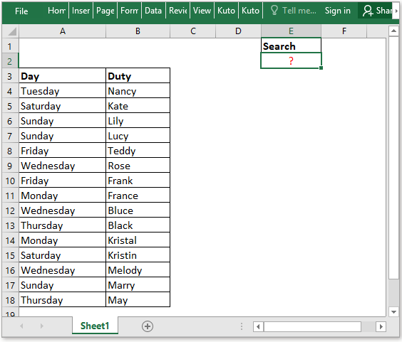
Suppose you have a data set and a dedicated cell for search input (as illustrated in the following screenshot). Here’s how you can set up conditional formatting to highlight matches dynamically:
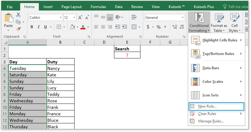
1. Select the entire range of cells where you want to search for your target value. Go to the Home tab, click Conditional Formatting, and then select New Rule.
2. In the New Formatting Rule dialog, choose Use a formula to determine which cells to format. Enter the following formula in the “Format values where this formula is true” box (replace cell references as needed):
=AND($E$2<>"",$E$2=A4)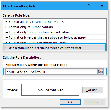
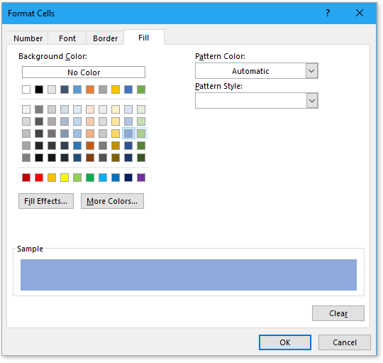
3. Click the Format button to open the Format Cells dialog box, then select a fill color of your choice on the Fill tab. Confirm with OK, and close any dialog windows.
Now, whenever you type a keyword in cell E2, the matching entries within your chosen range will be highlighted automatically. This process instantly updates when the search value changes, offering a seamless way to review data or search for terms repeatedly without manual adjustments.
Some useful notes:
• Conditional formatting formulas can handle both exact and partial matches (using SEARCH or FIND functions in more complex rules).
• This method is non-destructive—the underlying data remains unchanged.
• When copying conditional formatting to other areas, double-check cell references for accuracy (use absolute or relative references as needed).
• If the conditional formatting seems not to work, verify your formula and ensure the target cell for input is referenced correctly; errors usually relate to misplacement of the formula or overlap in range selections.
One limitation is that Conditional Formatting is limited to formatting and cannot, for example, filter, select, or otherwise manipulate the found results beyond visual cues. For interactive or persistent color-coding (such as across multiple sheets or workbooks), the VBA or Kutools solution may be more suitable.
If you often search for multiple values at once, or need an out-of-the-box solution for complex highlighting, the "Mark Keyword" feature found in Kutools for Excel offers unique flexibility. Unlike standard Excel features, Kutools allows you to input several keywords, specify a variety of highlight options, choose to match partial strings, and even make searches case-sensitive. This is particularly useful for quality control, auditing, or quickly marking multiple items in lists such as product IDs, client names, or other identifiers across large datasets.
To use this feature, proceed as follows:
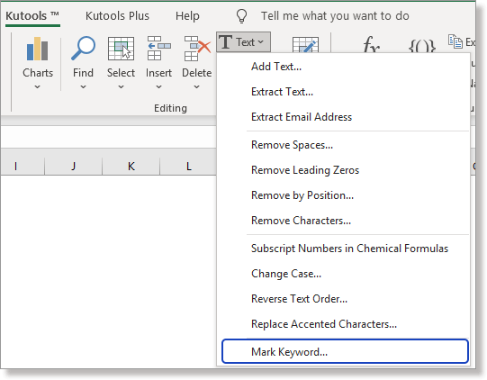
1. Select the range where you want to search for keywords. Then navigate to the Kutools tab, click Text, and choose Mark Keyword.
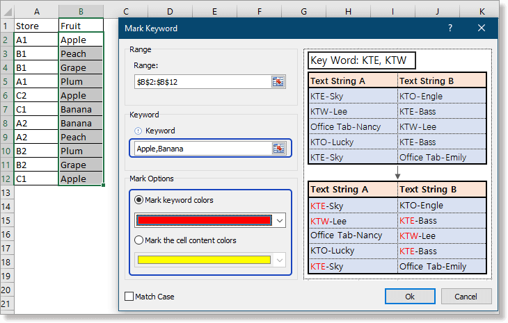
2. In the pop-up dialog, enter the words you want to search for in the “Keyword” box, separating each value with a comma. Select your preferred mark options—such as highlight color and font color—and specify how the match should occur (whole or part of string, and case sensitivity). Click OK to apply.
For example, check the “Match Case” box if you want to find only those entries that match the capitalization you enter. This is particularly useful when being precise about case is important, like searching for specific codes or product IDs.
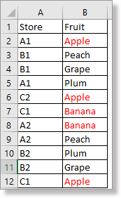
Very quickly, matched results within your selected range will be marked as specified, immediately drawing your attention to key entries. If you input multiple keywords, each occurrence will be highlighted throughout your data.
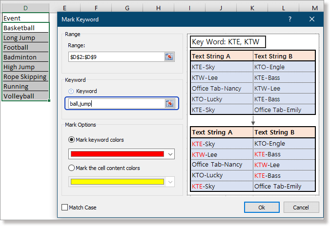
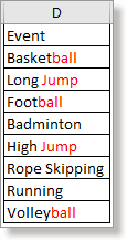
Additionally, the “Mark Keyword” feature permits partial string matching. For example, if you want to highlight all cells containing either “ball” or “jump”, simply type ball, jump into the Keyword box, choose your settings, and click OK.
 >>>
>>> 
This approach is straightforward and ideal for repetitive search and highlight tasks—saving significant time over manual formatting or creating complex conditional formatting rules. Kutools operations are easily accessible and revertible, and its marking options are highly customizable, making it well suited for high-volume data work.
Note that Kutools for Excel is an add-in and may require separate installation. After installation, it integrates directly into the Excel ribbon. For users seeking even more customization or simplicity for complex, multi-keyword scenarios, this feature is especially beneficial.
Kutools for Excel - Supercharge Excel with over 300 essential tools, making your work faster and easier, and take advantage of AI features for smarter data processing and productivity. Get It Now
In situations where you prefer not to use formulas, VBA, or third-party add-ins, you can use Excel's built-in Filter feature to narrow down your data to matching results, and then apply manual highlighting. This approach is straightforward and does not require any setup or risk of altering data structures.
Suitable for occasional tasks or when sharing files with users who may not have permissions for macros or add-ins, the steps are as follows:
- Select your data range (including headers, if available).
- Go to Data > Filter. Dropdown arrows will appear in the header row.
- Click the filter dropdown arrow for the column you want to search, and either use the Search box or select your value from the list. Click OK to filter the data.
- Once only the matching rows are visible, select these rows, go to the Home tab, and use the Fill Color tool to highlight them as needed.
- Clear the filter to see all data, with highlighted cells now easily identifiable.
Be mindful that this method is manual—if your dataset changes, you’ll need to repeat the filtering and highlighting steps. However, it works in all Excel versions and is especially practical for quick, one-time highlight needs or when macros are not allowed.
For users who want a reusable, easily auditable solution without using VBA or add-ins, using a simple formula in a helper column can quickly identify matches, which you can then highlight manually or with conditional formatting.
For example, suppose you are searching for a value in cell E2 within the range A4:A20. Do the following:
1. In the column next to your data (for instance, cell B4), enter the following formula:
=IF(A4=$E$2,"Match","")2. Press Enter. Copy the formula down to all relevant rows (e.g., B4:B20). This formula checks if the value in column A matches your search term and outputs "Match" if they are the same.
3. You can now filter the helper column to show only rows with "Match," or use conditional formatting to automatically highlight those rows based on the helper column value.
💡 Tip: To support partial matches, replace the equality check with this formula:
=IF(ISNUMBER(SEARCH($E$2,A4)),"Match","")This highlights rows if the search value is found anywhere within the cell. Remember to adjust absolute and relative references as needed.
Using a helper column keeps your data organized and makes it easy to audit or modify search logic later.
When choosing a method for searching and highlighting in Excel, consider your data size, sharing requirements, and need for automation. Macros are efficient but require permissions; conditional formatting is dynamic but may be limited to simple rules. Add-ins like Kutools offer advanced batch processing. Always keep your original data backed up before applying bulk formatting or running unfamiliar code. If you run into issues, double-check cell references, formula syntax, and, if using macros, make sure they are enabled and the workbook is saved before proceeding.
Sample File
Click to download the sample file
Count/sum cells by colors with conditional formatting in Excel
Now this tutorial will tell you some handy and easy methods to quickly count or sum the cells by color with conditional formatting in Excel.
Create a chart with conditional formatting in Excel
For example, you have a score table of a class, and you want to create a chart to color scores in different ranges, here this tutorial will introduce the method on solving this job.
Conditional formatting stacked bar chart in Excel
This tutorial, it introduces how to create conditional formatting stacked bar chart as below screenshot shown step by step in Excel.
Conditional formatting rows or cells if two columns equal in Excel
In this article, I introduce the method on conditional formatting rows or cells if two columns equal in Excel.
Apply conditional formatting for each row in Excel
Sometimes, you may want to apply the conditional formatting for per row. Except repeatedly setting the same rules for per row, there are some tricks on solving this job.
Best Office Productivity Tools
Supercharge Your Excel Skills with Kutools for Excel, and Experience Efficiency Like Never Before. Kutools for Excel Offers Over 300 Advanced Features to Boost Productivity and Save Time. Click Here to Get The Feature You Need The Most...
Office Tab Brings Tabbed interface to Office, and Make Your Work Much Easier
- Enable tabbed editing and reading in Word, Excel, PowerPoint, Publisher, Access, Visio and Project.
- Open and create multiple documents in new tabs of the same window, rather than in new windows.
- Increases your productivity by 50%, and reduces hundreds of mouse clicks for you every day!
All Kutools add-ins. One installer
Kutools for Office suite bundles add-ins for Excel, Word, Outlook & PowerPoint plus Office Tab Pro, which is ideal for teams working across Office apps.
- All-in-one suite — Excel, Word, Outlook & PowerPoint add-ins + Office Tab Pro
- One installer, one license — set up in minutes (MSI-ready)
- Works better together — streamlined productivity across Office apps
- 30-day full-featured trial — no registration, no credit card
- Best value — save vs buying individual add-in