Conditional formatting rows or cells if two columns equal in Excel
In Excel, comparing two columns and quickly identifying where their entries are equal is a common need, especially when you’re dealing with large datasets, data validation tasks, or reconciliation jobs. You may wish to highlight matching cells or entire rows to easily spot these matches visually, or you might want to process or select equal values directly. This tutorial provides multiple practical methods to highlight or select rows or cells if two columns contain the same values. Below, you’ll find a summary of the available solutions. Each method suits different use cases—choose the one that fits you best.
When working with data in Excel, it's often helpful to highlight the cells or rows where two columns contain equal values. Excel’s Conditional Formatting allows you to shade those matching areas automatically. This visual cue helps make data comparison more efficient and reduces the risk of missing matches, especially in large datasets.
This solution is suitable when you want a purely visual indicator to highlight equality between two columns. It adjusts dynamically as your data changes. However, it does not let you automatically select the matching cells for further processing. Here’s how you can set it up:
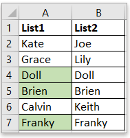
1. Select the first list of data that you want to compare with the second one. For example, choose range A2:A7. Then, from the ribbon, click Home > Conditional Formatting > New Rule.
2. In the New Formatting Rule dialog, choose Use a formula to determine which cells to format from Select a Rule Type. In the text box under Format values where this formula is true, enter =$A2=$B2.
Tip: Here, A2 and B2 are the starting cells for your two columns. Ensure your formula uses the correct cell references for your range. For example, if your data starts from row3, adjust the formula accordingly.
3. Click the Format button in the New Formatting Rule dialog. Choose a background color in the Fill tab of the Format Cells dialog to visually mark matching cells.
4. Click OK > OK to apply your changes. Excel will now automatically shade the cells where the values in the two columns are equal. This formatting will update dynamically if your data changes.
Tip: If you wish to highlight the entire row (not just the cell) when the two columns are equal, first select the combined data range for both columns (for example, A2:B7). Then, repeat the above steps, ensuring your formula fits the entire row. This will fill the row’s cells when the criteria are met.
Formula-based conditional formatting is ideal where you want a continuous, dynamic highlight as your data changes, but may not be suitable if you need to process or extract the equal values. In such cases, consider the other solutions below.
In some scenarios, you may wish not only to highlight matching cells, but also to select them for further processing (such as copying, formatting, or analysis). The Compare Cells feature of Kutools for Excel makes this much more efficient than built-in options.
After free installing Kutools for Excel, you can quickly identify, highlight, and optionally select matching cells between two columns. This method is especially valuable when you need to take further action after identifying matching data, and it provides flexibility in formatting results directly in the worksheet.
1. Select the first list, then select the second list while holding the Ctrl key. Next, choose Kutools > Compare Cells to open the Compare Cells dialog.
2. In the Compare Cells dialog, check the Same cells option. Also, check Fill backcolor or Fill font color and choose your preferred highlight color.
3. Click OK. The cells in both columns that are equal will now be selected and highlighted from the first list. This enables you to directly process, copy, or analyze only these cells.
Compared to conditional formatting, Kutools also provides the added capability to select equal cells—a major advantage for advanced data tasks.
If your workflow has additional requirements—such as automatically performing actions when two columns are equal (beyond the limitations of built-in formatting and selection)—a simple VBA macro can provide customization and automation. This approach is suitable for users who want to highlight cells, select rows, or take further steps like copying, deleting, or marking matching records, and is particularly valuable when regularly dealing with large or dynamic data sets.
1. Click Developer > Visual Basic. In the new Microsoft Visual Basic for Applications window, choose Insert > Module. Enter the following code into the module window:
Sub HighlightMatchingSelection()
    Dim rng       As Range
    Dim cell1     As Range, cell2 As Range
    Dim i         As Long
    On Error Resume Next
    Set rng = Application.InputBox( _
        Prompt:="Please select the two-column range to compare:", _
        Title:="Kutools for Excel", Type:=8)
    On Error GoTo 0
    If rng Is Nothing Then Exit Sub
    If rng.Columns.Count <> 2 Then
        MsgBox "You must select exactly two adjacent columns.", vbExclamation
        Exit Sub
    End If
    Application.ScreenUpdating = False
    For i = 1 To rng.Rows.Count
        Set cell1 = rng.Cells(i, 1)
        Set cell2 = rng.Cells(i, 2)
        If CStr(cell1.Value) = CStr(cell2.Value) Then
            cell1.Interior.Color = vbYellow
            cell2.Interior.Color = vbYellow
        Else
            cell1.Interior.ColorIndex = xlColorIndexNone
            cell2.Interior.ColorIndex = xlColorIndexNone
        End If
    Next i

    Application.ScreenUpdating = True

    MsgBox "Highlighting complete for " & rng.Rows.Count & " rows.", vbInformation
End Sub 2. To run the macro, click the ![]() button on the VBA editor toolbar, or press F5. In the prompt box, select the two columns, then, click OK button.
button on the VBA editor toolbar, or press F5. In the prompt box, select the two columns, then, click OK button.
Result: Cells with matching values in the two columns will be highlighted in yellow.
Another practical approach is to use a helper column to evaluate whether two columns are equal on each row. This method is very flexible: it allows you not only to visually see matches but also to sort, filter, or perform further processing such as extracting, deleting, or exporting rows. It is ideal for users who want to work with matching data programmatically or build more advanced logic on top of the results.
1. In a new helper column (for example, column C), enter the following formula in cell C2:
=A2=B22. Press Enter. The result will show as TRUE if the values in columns A and B are equal on that row, or FALSE if not.
3. Copy the formula down the helper column to the end of your data by dragging the fill handle or double-clicking it.
4. Once all results are generated, you can use Excel’s Filter feature (Data > Filter) to display only rows where the helper column is TRUE (i.e., where two columns match). You can also sort, delete unmatched rows, or carry out further analysis as needed.
Sample File
Count/sum cells by colors with conditional formatting in Excel
Now this tutorial will tell you some handy and easy methods to quickly count or sum the cells by color with conditional formatting in Excel.
create a chart with conditional formatting in Excel
For example, you have a score table of a class, and you want to create a chart to color scores in different ranges, here this tutorial will introduce the method on solving this job.
Apply conditional formatting for each row
Sometimes, you may want to apply the conditional formatting for per row, except repeatedly setting the same rules for per row, there are some tricks on solving this job.
Conditional formatting stacked bar chart in Excel
This tutorial, it introduces how to create conditional formatting stacked bar chart as below screenshot shown step by step in Excel.
Search and highlight search results in Excel
In Excel, you can use the Find and Replace function to find a specific value, but do you know how to highlight the search results after searching? In this article, I introduce two different ways to help you search and highlight search results at the meanwhile in Excel.
The Best Office Productivity Tools
Kutools for Excel Solves Most of Your Problems, and Increases Your Productivity by 80%
- Super Formula Bar (easily edit multiple lines of text and formula); Reading Layout (easily read and edit large numbers of cells); Paste to Filtered Range...
- Merge Cells/Rows/Columns and Keeping Data; Split Cells Content; Combine Duplicate Rows and Sum/Average... Prevent Duplicate Cells; Compare Ranges...
- Select Duplicate or Unique Rows; Select Blank Rows (all cells are empty); Super Find and Fuzzy Find in Many Workbooks; Random Select...
- Exact Copy Multiple Cells without changing formula reference; Auto Create References to Multiple Sheets; Insert Bullets, Check Boxes and more...
- Favorite and Quickly Insert Formulas, Ranges, Charts and Pictures; Encrypt Cells with password; Create Mailing List and send emails...
- Extract Text, Add Text, Remove by Position, Remove Space; Create and Print Paging Subtotals; Convert Between Cells Content and Comments...
- Super Filter (save and apply filter schemes to other sheets); Advanced Sort by month/week/day, frequency and more; Special Filter by bold, italic...
- Combine Workbooks and WorkSheets; Merge Tables based on key columns; Split Data into Multiple Sheets; Batch Convert xls, xlsx and PDF...
- Pivot Table Grouping by week number, day of week and more... Show Unlocked, Locked Cells by different colors; Highlight Cells That Have Formula/Name...
")
- Enable tabbed editing and reading in Word, Excel, PowerPoint, Publisher, Access, Visio and Project.
- Open and create multiple documents in new tabs of the same window, rather than in new windows.
- Increases your productivity by 50%, and reduces hundreds of mouse clicks for you every day!
")