How to VLOOKUP and Return All Matches Horizontally in Excel
When a lookup value appears more than once in Excel, a standard VLOOKUP normally returns only the first matching result. However, many datasets contain multiple related records. For example, one customer may have several Order IDs, one department may contain multiple employees, or one category may include several products.
Vlookup and return all corresponding values horizontally in Kutools for Excel's Formula Helper Plus helps retrieve all matching values and arrange them horizontally across adjacent cells. Instead of manually building a complex formula with INDEX, SMALL, IF, ROW, and COLUMN, you specify the lookup criteria and related ranges, and Formula Helper Plus creates the formula for you.
Advantages of Vlookup and return all corresponding values horizontally
How to VLOOKUP and return all matching values horizontally
- Return all matching values horizontally with Formula Helper Plus
- Understand the four formula arguments
- How the generated INDEX, SMALL, IF, and COLUMN formula works
Standard VLOOKUP vs. returning all matches horizontally
Advantages of Vlookup and return all corresponding values horizontally
Vlookup and return all corresponding values horizontally is useful when one lookup value can correspond to several records and you need to retrieve all of them rather than only the first match.
Return every matching value
Retrieve multiple corresponding records when the same lookup value appears more than once, instead of stopping at the first match.
Arrange multiple results horizontally
Return the first, second, third, and subsequent matches across adjacent columns, making related results easy to review in one row.
Avoid building a complex formula manually
Formula Helper Plus creates the required INDEX, SMALL, IF, ROW, COLUMN, and IFERROR structure after you specify the required ranges.
Configure the lookup through labeled arguments
Separate fields for the output range, lookup criterion, criteria range, and starting lookup cell make the formula easier to configure and understand.
How to VLOOKUP and return all matching values horizontally
Vlookup and return all corresponding values horizontally finds every record that matches a specified criterion and returns the related values across adjacent columns. This section shows how to locate the formula, configure its four arguments, and understand how the generated formula retrieves multiple matches.
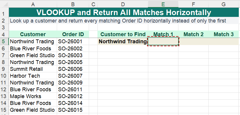
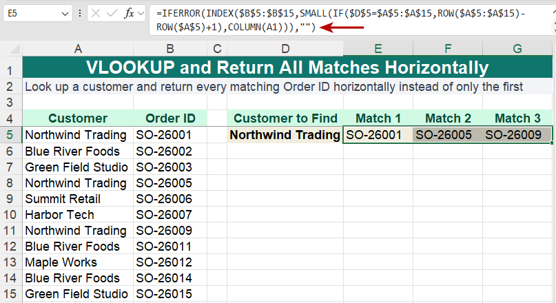
In the example below, a customer may have several orders. Northwind Trading is used as the lookup value, and all corresponding Order IDs are returned horizontally.
Return all matching values horizontally with Formula Helper Plus
Use this method when one lookup value appears multiple times and you want to retrieve every corresponding value in the order in which the records appear in the source data.
1. Prepare the source data and lookup area. In this example, customer names are stored in A5:A15, Order IDs are stored in B5:B15, and the customer to find, Northwind Trading, is entered in D5. Select E5, where you want the first matching Order ID to appear.
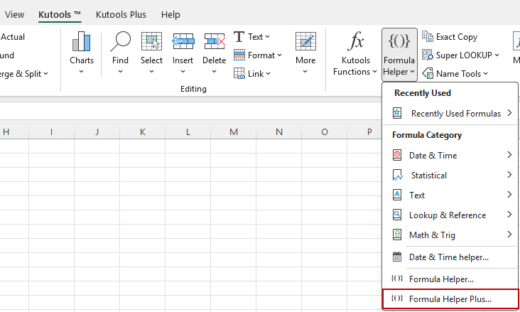
2. Click Kutools > Formula Helper > Formula Helper Plus.
3. In Formula Helper Plus, select the Online tab. Under Category, click Lookup, then select Vlookup and return all corresponding values horizontally.
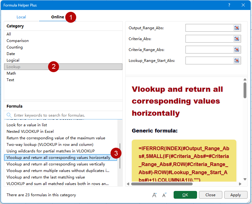
Tip: You can also enter keywords such as return all corresponding values or Vlookup horizontally in the search box to quickly locate the formula.
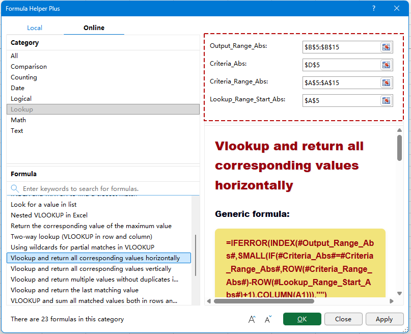
4. Specify the four arguments. Select B5:B15 as Output_Range_Abs, D5 as Criteria_Abs, A5:A15 as Criteria_Range_Abs, and A5 as Lookup_Range_Start_Abs.
5. Click OK or Apply to insert the formula into E5. Then drag the fill handle to the right to return the second, third, and subsequent matches.
Result: All Order IDs matching Northwind Trading are returned horizontally across adjacent cells. Once there are no more matches, the remaining cells return blank.
Tip: Fill the formula far enough to the right to accommodate the maximum number of possible matches. Once there are no more matching records, the formula returns blank cells rather than errors.
Understand the four formula arguments
The formula uses four arguments to identify the lookup value, find matching records, and return the corresponding results.
| Argument | Purpose | Example |
| Output_Range_Abs | The range containing the values you want to return for matching records. | B5:B15 — Order ID |
| Criteria_Abs | The lookup value used to identify matching records. | D5 — Northwind Trading |
| Criteria_Range_Abs | The range in which Excel searches for the lookup value. | A5:A15 — Customer |
| Lookup_Range_Start_Abs | The first cell of the lookup range, used as the starting reference for calculating relative row positions. | A5 |
Tip:Output_Range_Abs and Criteria_Range_Abs should cover corresponding records and contain the same number of rows. Lookup_Range_Start_Abs should normally be the first cell of the criteria range.
How the generated INDEX, SMALL, IF, and COLUMN formula works
The generic formula used by Vlookup and return all corresponding values horizontally is:
=IFERROR(INDEX(#Output_Range_Abs#,SMALL(IF(#Criteria_Abs#=#Criteria_Range_Abs#,ROW(#Criteria_Range_Abs#)-ROW(#Lookup_Range_Start_Abs#)+1),COLUMN(A1))),"")With the cell references used in this example, the generated formula follows this structure:
=IFERROR(INDEX($B$5:$B$15,SMALL(IF($D$5=$A$5:$A$15,ROW($A$5:$A$15)-ROW($A$5)+1),COLUMN(A1))),"")The formula works in several stages:
- $D$5=$A$5:$A$15 checks each customer name and identifies the rows that match Northwind Trading.
- ROW($A$5:$A$15)-ROW($A$5)+1 converts the matching worksheet rows into relative positions within the lookup range.
- SMALL retrieves the first, second, third, and subsequent matching positions.
- INDEX uses each matching position to return the corresponding Order ID from B5:B15.
- COLUMN(A1) supplies 1 in the first result cell. When the formula is copied to the right, it becomes COLUMN(B1), COLUMN(C1), and so on, allowing the formula to retrieve the second, third, and later matches.
- IFERROR returns a blank once there are no additional matches instead of displaying an error.
For example, the first formula returns SO-26001. After the formula is filled to the right, the next cells return SO-26005, and SO-26009.
Key point: Although the feature name refers to VLOOKUP, the generated formula uses INDEX together with SMALL, IF, ROW, and COLUMN so that it can return multiple matching values rather than only the first match.
Standard VLOOKUP vs. returning all matches horizontally
A standard VLOOKUP is useful when you only need one corresponding value. When the lookup value appears several times, however, it normally stops at the first match.
| Method | Lookup Value | Result |
| Standard VLOOKUP | Northwind Trading | SO-26001 |
| Vlookup and return all corresponding values horizontally | Northwind Trading | SO-26001 | SO-26005 | SO-26009 |
The Formula Helper Plus method is therefore especially useful when one lookup value can be associated with several records, and you need to see all of them together.
Tips for accurate multiple-match lookups
Keep the following points in mind when returning multiple matching values horizontally.
- Keep the criteria and output ranges aligned:Criteria_Range_Abs and Output_Range_Abs should cover corresponding records and contain the same number of rows.
- Use the first lookup cell as the starting reference:Lookup_Range_Start_Abs should normally point to the first cell in Criteria_Range_Abs.
- Keep lookup values consistent: Extra spaces or inconsistent text may prevent values that look identical from matching correctly.
- Leave enough cells to the right: Because each additional match is returned in the next column, make sure the result area has enough empty cells for all expected matches.
- Fill the formula far enough: Copy the generated formula across enough columns to retrieve all possible matches. Cells after the final matching result remain blank.
- Results follow the source order: Matches are returned according to their position in the original criteria range, from top to bottom.
Practical use cases
This lookup method is useful whenever one value can be associated with multiple related records.
Return all orders for one customer
Look up a customer name or Customer ID and return every related Order ID horizontally for quick review.
Return all products in one category
Look up a product category such as Accessories and return all corresponding product names across one row.
Return all employees in one department
Use a department such as Sales as the criterion and return every employee assigned to that department.
Return all invoices for one supplier
Look up a supplier and retrieve all related invoice numbers without manually filtering the source table.
Return all projects assigned to one manager
Use a manager name as the lookup criterion and display all corresponding project names horizontally.
About Formula Helper Plus
Formula Helper Plus in Kutools for Excel provides a collection of practical formulas through a guided interface, helping you find, understand, and insert formulas without having to remember their complete syntax.
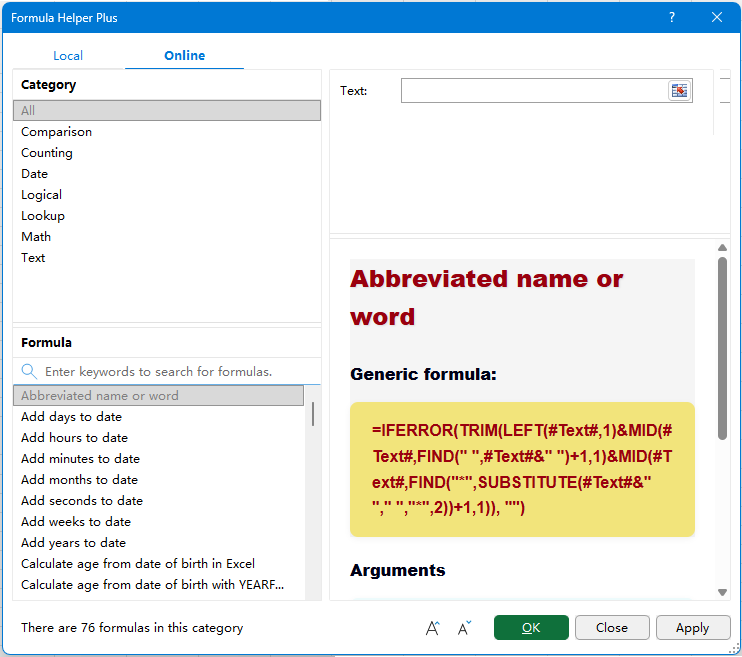
The interface includes Local and Online formula libraries. Formulas are organized by task, and you can browse categories or use the search box to quickly locate a formula by name or purpose. Vlookup and return all corresponding values horizontally is available in the Online library under the Lookup category.
After selecting a formula, its argument boxes appear at the top of the window, while the right-hand information pane displays the formula description, generic formula, argument explanations, and other guidance to help you configure the formula correctly.
🔤 Display controls
Use the display controls at the bottom of the Formula Helper Plus window to adjust the text size in the right-hand information pane for easier reading. These controls are available in both the Local and Online libraries.
 Increase font size: Enlarge the formula description, generic formula, arguments, and other information displayed in the right-hand pane.
 Decrease font size: Reduce the text size in the right-hand pane when you want to view more information at once.
 Increase font size: Enlarge the formula description, generic formula, arguments, and other information displayed in the right-hand pane.
 Decrease font size: Reduce the text size in the right-hand pane when you want to view more information at once.
FAQ
What does Vlookup and return all corresponding values horizontally do?
It finds every record that matches a specified lookup value and returns the corresponding values horizontally across adjacent columns.
How is this different from a standard VLOOKUP?
A standard VLOOKUP normally returns only the first matching value. This formula can return the first, second, third, and subsequent matches across multiple columns.
Do I need to fill the generated formula to the right?
Yes. After Formula Helper Plus inserts the first formula, fill or copy it to the right to retrieve additional matches. The COLUMN reference changes as the formula moves across columns, allowing each cell to return the next matching value.
What happens when there are no more matching values?
The formula uses IFERROR to return a blank after the final match, so extra result cells do not display an error.
Can the returned values be text or numbers?
Yes. Output_Range_Abs can contain text, numbers, IDs, dates, or other values that you want to return for the matching records.
Do Output_Range_Abs and Criteria_Range_Abs need to be the same size?
Yes. They should cover corresponding records and normally contain the same number of rows so that each criterion is aligned with the value to return.
What should I select for Lookup_Range_Start_Abs?
Select the first cell of the criteria range. For example, if Criteria_Range_Abs is A5:A16, use A5 as Lookup_Range_Start_Abs.
Are the matches returned in the same order as the source data?
Yes. The formula retrieves matching records from top to bottom based on their positions in the source range.
What happens if the lookup value appears only once?
The single matching value is returned first, and cells filled farther to the right remain blank because there are no additional matches.
What happens if there is no matching value?
The result remains blank because IFERROR suppresses the error that would otherwise occur when no matching position is found.
Where can I find Vlookup and return all corresponding values horizontally?
Click Kutools > Formula Helper > Formula Helper Plus, select the Online tab, and choose Lookup > Vlookup and return all corresponding values horizontally. You can also use the search box to locate the formula by keyword.
Productivity Tools Recommended
Office Tab: Use handy tabs in Microsoft Office, just like Chrome, Firefox, and the new Edge browser. Easily switch between documents with tabs — no more cluttered windows. Know more...
Kutools for Outlook: Kutools for Outlook offers 100+ powerful features for Microsoft Outlook 2010–2024 (and later versions), as well as Microsoft 365, helping you simplify email management and boost productivity. Know more...
Kutools for Excel
Kutools for Excel offers 300+ advanced features to streamline your work in Excel 2010 – 2024 and Microsoft 365. The feature above is just one of many time-saving tools included.

Table of Contents
- Advantages of Vlookup and return all corresponding values horizontally
- How to VLOOKUP and return all matching values horizontally
- Return all matching values horizontally with Formula Helper Plus
- Understand the four formula arguments
- How the generated INDEX, SMALL, IF, and COLUMN formula works
- Standard VLOOKUP vs. returning all matches horizontally
- Tips for accurate multiple-match lookups
- Practical use cases
- About Formula Helper Plus
- FAQ
- The Best Office Productivity Tools
Kutools for Excel
Brings 300+ advanced features to Excel
- 🧩 Overview
- 📥 Free Download
- 🎁 30-Day Free Trial available