Highlight the highest / lowest value in each row or column - 2 easy ways
When working with data spanning multiple columns and rows, manually identifying and highlighting the largest or smallest value in each row or column can be time-consuming. However, Excel offers efficient solutions through its features. This article will discuss some useful tricks in Excel to streamline this task, making it easier to highlight the highest or lowest values in each row or column.
Highlight highest / lowest value in each row or column with Conditional Formatting
Highlight highest / lowest value in each row or column with Kutools AI Aide
Highlight highest / lowest value in each row or column with Conditional Formatting
Excel's Conditional Formatting feature offers a solution to this challenge. By applying Conditional Formatting, you can automatically highlight the highest or lowest value in each row or column, making them visually stand out. Here’s a detailed guide on how to apply Conditional Formatting feature.
Highlight the highest / lowest value in each row:
- Select the range of cells where you want to highlight the highest or lowest values in each row.
- Then, click Home > Conditional Formatting > New Rule, see screenshot:

- In the New Formatting Rule dialog box:
- Click Use a formula to determine which cells to format from Select a Rule Type list box;
- Enter one of the following formulas you need:
● Highlight the highest value in each row:
● Highlight the lowest value in each row:=B2=MAX($B2:$E2)
=B2=MIN($B2:$E2) - Then, click Format button.

- In the Format Cells dialog box, please select one color you like under the Fill tab, see screenshot:

- And then, click OK > OK to close the dialogs, and you will see the largest or smallest value has been highlighted in each row.
Highlight the highest value in each row: Highlight the lowest value in each row: 


Highlight the highest / lowest value in each column:
To highlight the highest or lowest value in each column, please apply the following formula into the Conditional Formatting:
● Highlight the highest value in each column:
=B2=MAX(B$2:B$10)● Highlight the lowest value in each column:
=B2=MIN(B$2:B$10)After applying the formula into the Conditional Formatting, you will get the results as following screenshots shown:
| Highlight the highest value in each column: | Highlight the lowest value in each column: |
 |
 |
Highlight highest / lowest value in each row or column with Kutools AI Aide
Are you ready to take your data analysis in Excel to the next level? Introducing Kutools AI Aide, your ultimate solution for effortlessly highlighting the highest and lowest values in each row or column with precision and speed! Simply input your command, and watch as Kutools AI Aide delivers instant results, transforming your data handling experience with efficiency and ease.
After installing Kutools for Excel, please click Kutools AI > AI Aide to open the Kutools AI Aide pane:
- Select the data range, then type your requirement into the chat box, and click Send button or press Enter key to send the question;
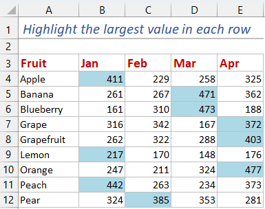
“Highlight the largest values in each row of the selection with light blue color:” - After analyzing, click Execute button to run. Kutools AI Aide will process your request using AI and highlight the largest value in each row directly in Excel.


- To highlight the lowest value in each row or highest / lowest value in each column, you just need to modify the command to your need. For example, use commands like "Highlight the lowest value in each row of the selection with light red color"
- This method does not support the undo function. However, if you wish to restore the original data, you can click Unsatisfied to revert the changes.
Related Articles:
- Highlight approximate match lookup
- In Excel, we can use the Vlookup function to get the approximate matched value quickly and easily. But, have you ever tried to get the approximate match based on row and column data and highlight the approximate match from the original data range as below screenshot shown? This article will talk about how to solve this task in Excel.
- Highlight cells if value greater or less than a number
- Let’s say you have a table with large amounts of data, to find the cells with values that are greater or less than a specific value, it will be tiresome and time-consuming. In this tutorial, I will talk about the ways to quickly highlight the cells that contain values greater or less than a specified number in Excel.
- Highlight winning lottery numbers in Excel
- To check a ticket if winning the lottery numbers, you can check it one by one number. But, if there are multiple tickets need to be checked, how could you solve it quickly and easily? This article, I will talk about highlighting the winning lottery numbers to check if win the lottery as below screenshot shown.
- Highlight rows based on multiple cell values
- Normally, in Excel, we can apply the Conditional Formatting to highlight the cells or rows based on a cell value. But, sometimes, you may need to highlight the rows based on multiple cell values. For example, I have a data range, now, I want to highlight the rows which product is KTE and order is greater than 100 as following screenshot shown. How could you solve this job in Excel as quickly as you can?
Best Office Productivity Tools
Supercharge Your Excel Skills with Kutools for Excel, and Experience Efficiency Like Never Before. Kutools for Excel Offers Over 300 Advanced Features to Boost Productivity and Save Time. Click Here to Get The Feature You Need The Most...
")
Office Tab Brings Tabbed interface to Office, and Make Your Work Much Easier
- Enable tabbed editing and reading in Word, Excel, PowerPoint, Publisher, Access, Visio and Project.
- Open and create multiple documents in new tabs of the same window, rather than in new windows.
- Increases your productivity by 50%, and reduces hundreds of mouse clicks for you every day!
")