How to vlookup matching value from bottom to top in Excel?
Normally, the Vlookup function can help you to find the data from top to bottom to get the first matching value from the list. But, sometimes, you need to vlookup from bottom to top to extract the last corresponding value. Do you have any good ideas to deal with this task in Excel?
Vlookup the last matching value from bottom to top with formula
Vlookup the last matching value from bottom to top with a useful feature
Vlookup the last matching value from bottom to top with formula
To vlookup matching value from bottom to top, the following LOOKUP formula can help you, please do as follows:
Please enter the below formula into a blank cell where you want to get the result:
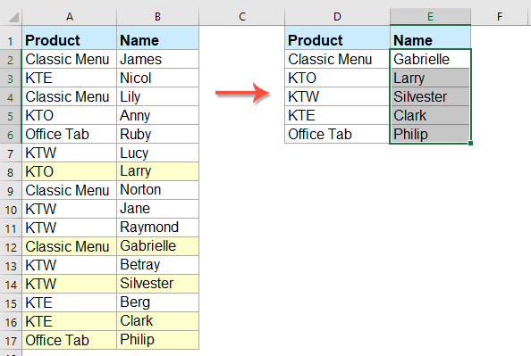
Then drag the fill handle down to the cells that you want to get the results, the last corresponding values will be returned at once, see screenshot:
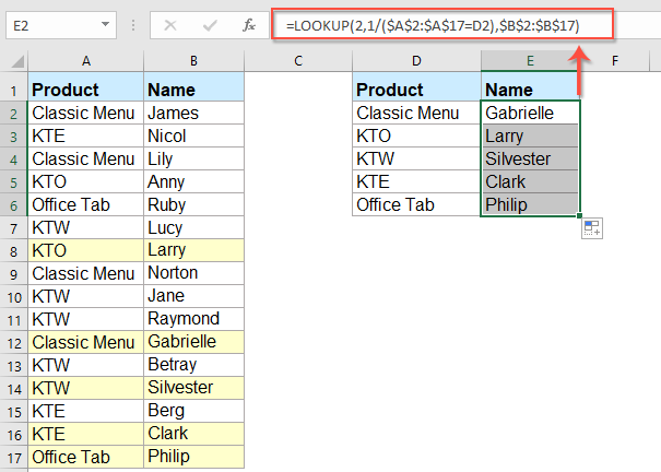
Note: In the above formula: A2:A17 indicates the column that you are looking for, D2 is the criteria which you want to return its relative data and B2:B17 is the list that contains the value you want to return.
Vlookup the last matching value from bottom to top with a useful feature
If you have Kutools for Excel, with its LOOKUP from Bottom to Top feature, you can also solve this task without remembering any formula.
Tips:To apply this LOOKUP from Bottom to Top feature, firstly, you should download the Kutools for Excel, and then apply the feature quickly and easily.
After installing Kutools for Excel, please do as this:
1. Click Kutools > Super LOOKUP > LOOKUP from Bottom to Top, see screenshot:

2. In the LOOKUP from Bottom to Top dialog box, do the following operations:
- Select the lookup value cells and output cells from the Lookup values and Output Range section;
- Then, specify the corresponding items from the Data range section.

3. Then, click OK button, all the last matching values will be returned at once, see screenshot:
Download and free trial Kutools for Excel Now!
More relative articles:
- Vlookup Values Across Multiple Worksheets
- In excel, we can easily apply the vlookup function to return the matching values in a single table of a worksheet. But, have you ever considered that how to vlookup value across multiple worksheet? Supposing I have the following three worksheets with range of data, and now, I want to get part of the corresponding values based on the criteria from these three worksheets.
- Use Vlookup Exact And Approximate Match In Excel
- In Excel, vlookup is one of the most important functions for us to search a value in the left-most column of the table and return the value in the same row of the range. But, do you apply the vlookup function successfully in Excel? This article, I will talk about how to use the vlookup function in Excel.
- Vlookup To Return Blank Or Specific Value Instead Of 0 Or N/A
- Normally, when you apply the vlookup function to return the corresponding value, if your matching cell is blank, it will return 0, and if your matching value is not found, you will get an error #N/A value as below screenshot shown. Instead of displaying the 0 or #N/A value, how can you make it show blank cell or other specific text value?
- Vlookup And Return Whole / Entire Row Of A Matched Value In Excel
- Normally, you can vlookup and return a matching value from a range of data by using the Vlookup function, but, have you ever tried to find and return the whole row of data based on specific criteria as following screenshot shown.
- Vlookup And Concatenate Multiple Corresponding Values In Excel
- As we all known, the Vlookup function in Excel can help us to lookup a value and return the corresponding data in another column, but in general, it can only get the first relative value if there are multiple matching data. In this article, I will talk about how to vlookup and concatenate multiple corresponding values in only one cell or a vertical list.
Best Office Productivity Tools
Supercharge Your Excel Skills with Kutools for Excel, and Experience Efficiency Like Never Before. Kutools for Excel Offers Over 300 Advanced Features to Boost Productivity and Save Time. Click Here to Get The Feature You Need The Most...
")
Office Tab Brings Tabbed interface to Office, and Make Your Work Much Easier
- Enable tabbed editing and reading in Word, Excel, PowerPoint, Publisher, Access, Visio and Project.
- Open and create multiple documents in new tabs of the same window, rather than in new windows.
- Increases your productivity by 50%, and reduces hundreds of mouse clicks for you every day!
")