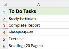
Strikethrough text in Excel features a line crossing through the text in a cell, signifying that the text is crossed out. This visual cue is beneficial for highlighting completed tasks or information that is no longer relevant.

In Excel, you can apply strikethrough through one of four basic methods (shortcut, Format Cells, add the strikethrough to QAT or Ribbon) presented in this tutorial. Additionally, the tutorial will include examples demonstrating the use of strikethrough in Excel.

Apply and remove strikethrough in Excel

• By using shortcut
• By using Format Cells feature
• Add the strikethrough icon to Quick Access Toolbar
• Add the strikethrough option to Excel ribbon
• Remove strikethrough

4 examples of strikethrough in Excel

• Example 1: Auto strikethrough based on cell value
• Example 2: Auto strikethrough when checkbox is checked
• Example 3: Double click a cell to strikethrough text
• Example 4: Apply strikethrough to multiple cells of the same text

Apply and remove strikethrough in Excel on Web

Apply and remove strikethrough in Excel on Mac

FAQs about strikethrough

Video: Strikethrough text in Excel (Basic usages and examples)

 Apply and remove strikethrough in Excel

While Excel doesn't have a direct strikethrough button like Word, there are several easy methods to apply or remove this format. Let's explore these methods:

Apply strikethrough by using shortcut

One of the quickest ways to apply strikethrough in Excel is by using a keyboard shortcut. This shortcut for strikethrough can be applied to a whole cell, a certain part of text within a cell, or across a selection of multiple cells.

The shortcut to strikethrough in Excel is: 

Ctrl + 5

● Add strikethrough to a cell:

Select the cell and then press the shortcut keys:

● Add strikethrough to a range of cells:

Select the range of cells and then press the shortcut keys:

● Add strikethrough to non-adjacent cells:

Press Ctrl key to select multiple cells and then press the shortcut keys:

● Add strikethrough to part of the cell value:

Double-click the cell to enable the edit mode and select the text you want to strikethrough, and then press the shortcut keys:

Amazing! Using Efficient Tabs in Excel Like Chrome, Edge, Firefox and Safari!
Save 50% of your time, and reduce thousands of mouse clicks for you every day!

Apply strikethrough by using Format Cells feature

If you prefer using menu options, the Format Cells feature is a great alternative.

Step 1: Select the cells or part of the text in a cell you want to apply strikethrough

Step 2: Go to the Format Cells dialog box

1. Right click the selected cell or text, and then choose Format Cells from the context menu.
2. In the Format Cells dialog box, under the Font tab, check Strikethrough option from the Effects section.
3. Click OK to close the dialog box.
   

Result:

Now, you can see that the selected cells have been formatted with strikethrough as shown in the following screenshot:

Add the strikethrough icon to Quick Access Toolbar

If you frequently use the Strikethrough feature in Excel, the method of navigating through menus each time can become cumbersome. This section introduces a more efficient solution: adding a Strikethrough button directly to your Quick Access Toolbar. This will streamline your workflow in Excel, allowing for immediate access to the strikethrough function with just a click.

Step-by-Step guide to add the Strikethrough icon:

1. Click on the small arrow at the end of the Quick Access Toolbar in the upper left corner of the Excel window, and then click More Commands, see screenshot:
   
2. In the Excel Options dialog box, set the following operations:
   • (1.) Under Choose commands from section, select Commands Not in the Ribbon;
   • (2.) Scroll through the list and select Strikethrough;
   • (3.) Click Add button to add Strikethrough to the list of commands on the right pane;
   • (4.) Finally, click OK button.
     

The strikethrough icon will now appear on your Quick Access Toolbar. See screenshot:

Now, when you need to add strikethrough to cells, just select the cells, and then click this Strikethrough icon, it will strikethrough the selected cells, as shown the demo below:

Add the strikethrough option to Excel ribbon

If the Strikethrough feature isn't used frequently enough to warrant a spot on your Quick Access Toolbar, but still is a tool you use regularly, adding it to the Excel Ribbon is a great alternative. Here will introduce the steps to add Strikethrough to the Excel Ribbon.

Step 1: Assess Excel Options dialog

Right-click anywhere on the Ribbon and select Customize the Ribbon, see screenshot:

Step 2: Create a new group

1. In the Excel Options dialog box, please create a new group under the Home tab. Select the Home tab, and click New Group, then, then click Rename button, see screenshot:
   
2. In the Rename dialog, type a name for the new group, and then, click OK. See screenshot:
   

Step 3: Add Strikethrough to the ribbon

1. Still in the Excel Options dialog box, set the following operations:
   • (1.) Under Choose commands from section, select Commands Not in the Ribbon.
   • (2.) Scroll through the list and select Strikethrough.
   • (3.) Click Add button to add Strikethrough to the new group on the right pane.
     
2. Change the new group position, select the new group you have created, and click the Up-arrow button to adjust it to the position you need. And then, click OK button.
   
3. Now, you can see that the new group, which includes the Strikethrough option, has been added under the Home tab, see screenshot:
   

Result:

From now on, when adding strikethrough to cells, just select the cells, and click this Strikethrough command, it will strikethrough the selected cells, as shown the demo below:

Remove strikethrough in Excel

This section will talk about two normal tricks to remove strikethrough from cells in Excel.

Option 1: By using shortcut

Select the cells with strikethrough formatting and simply press Ctrl + 5 again. The strikethrough will be removed at once.

Option 2: By using Format Cells feature

Select the cells with strikethrough formatting, and then right click, then choose Format Cells from the context menu. In the Format Cells dialog box, under the Font tab, uncheck the Strikethrough option. Finally, click OK. See screenshot:

 4 examples of strikethrough in Excel

Strikethrough in Excel is not just a static formatting option; it can be dynamically applied to enhance data management and user interaction. This section delves into four practical examples where strikethrough is used, demonstrating the flexibility and utility of this feature in various scenarios.

Example 1: Auto strikethrough based on cell value

If you're considering using strikethrough to mark off completed tasks or activities in a checklist or to-do list, automating this process in Excel can be highly efficient. You can set up Excel to automatically apply strikethrough formatting to tasks as soon as you enter a specific text, such as "Done" in a related cell. See the demo below:

Step 1: Select the data range where you want the auto strikethrough to apply

Step 2: Apply the Conditional Formatting feature

1. Navigate to the Home tab and click Conditional Formatting > New Rule, see screenshot:
   
2. In the New Formatting Rule dialog box:
   • (1.) Click Use a formula to determine which cells to format from the Select a Rule Type list box;
   • (2.) Type the below formula into the Format values where this formula is true textbox:

     =$B2="Done"

   • (3.) Then, click Format button.
      Note: In the above formula, B2 is the cell which contains the specific value, and Done is the text that you want to apply the strikethrough format based on.
     
3. In the popped-out Format Cells dialog box, under the Font tab, check Strikethrough option from the Effects section, see screenshot:
   
4. Then, click OK > OK to close the dialogs.

Result:

Now, when you type the text “Done” in the cells of Column B, the task item will be crossed out by a strikethrough, see the demo below:

Example 2: Auto strikethrough when checkbox is checked

Instead of typing text, using checkboxes to automatically apply strikethrough to tasks is also a great method for easily seeing which activities are done. This approach not only simplifies keeping track of what's completed but also makes your spreadsheets more interactive and user-friendly. See the following demo:

Step 1: Insert Checkboxes

1. Go to the Developer tab, select Insert, and then click Check Box from the Form Controls.
   
2. Click on the cell where you want the checkbox to appear and draw it.
   
3. Then, right click the check box, and choose Edit Text, then you can edit the checkbox to remove the text.
   
4. After removing the text of the checkbox, select the cell contains the check box, and then drag the fill handle down to fill the checkboxes, see screenshot:
   

Step 2: Link the checkboxes to cells

1. Right-click on the first checkbox and select Format Control, see screenshot:
   
2. In the Format Object dialog box, under the Control tab, link the checkbox to a cell (e.g., the cell right next to it, here is cell C2). Then, click OK button. See screenshot:
   
3. Repeat the above two steps to individually link each check box to the cell next to it. The linked cell will show TRUE when the checkbox is checked and FALSE when it's unchecked. See screenshot:
   

Step 3: Applying Conditional Formatting feature

1. Select the range of tasks you want to apply strikethrough formatting to.
2. Go to Home > Conditional Formatting > New Rule to open the New Formatting Rule dialog box.
3. In the New Formatting Rule dialog box:
   • (1.) Click Use a formula to determine which cells to format from the Select a Rule Type list box;
   • (2.) Type the below formula into the Format values where this formula is true textbox:

     =$C2=True

   • (3.) Then, click Format button.
      Note: In the above formula, C2 is the cell which is a cell which linked to the check box.
     
4. In the Format Cells dialog box, under the Font tab, check Strikethrough option from the Effects section, see screenshot:
   
5. Then, click OK > OK to close the dialogs.

Result:

Now, when you check a checkbox, the corresponding task item will automatically be formatted with a strikethrough. See the demo below:

Example 3: Double click a cell to strikethrough text

Using a double-click to toggle strikethrough formatting streamlines the process of marking tasks or items as complete or pending. This approach is particularly beneficial for to-do lists, project trackers, or any scenario where quick status updates are essential. This section provides a step-by-step guide on how to double click a cell to strikethrough text in Excel.

Step 1: Open the worksheet where you want to double click to strikethrough text

Step 2: Open the VBA sheet module editor and copy the code

1. Right click the sheet name, and choose View Code from the context menu, see screenshot:
   
2. In the opened VBA sheet module editor, copy and paste the following code into the blank module. See screenshot:
   VBA code: double click to strikethrough text

   Private Sub Worksheet_BeforeDoubleClick(ByVal Target As Range, Cancel As Boolean)
       'Update by Extendoffice
       With Target
           .Font.Strikethrough = Not .Font.Strikethrough
       End With
       Cancel = True
   End Sub
   

   
3. Then, close the VBA editor window to return to the worksheet.

Result:

Now, by double-clicking a cell containing text, you'll apply a strikethrough to its contents. Double-clicking the same cell again will remove the strikethrough formatting. See the demo below:

Example 4: Apply strikethrough to multiple cells of the same text

Applying a consistent strikethrough to repeated text entries helps in identifying patterns, changes, or completion statuses across a dataset. It's particularly useful in a large worksheet where manual formatting can be time-consuming and prone to errors. This section provides a useful way on how to efficiently apply strikethrough to multiple cells containing the same text.

Step 1: Select the range of cells you want to apply strikethrough

Step 2: Apply the Find and Replace feature

1. Click Home > Find & Select > Replace, (or press Ctrl + H ) to open the Find and Replace dialog box, see screenshot:
   
2. In the Find and Replace dialog box:
   • (1.) In the Find what field, enter the text you wish to apply strikethrough formatting to.
   • (2.) Then, click on the Format button located in the Replace with field.
   • (3.) And then choose Format from the drop down.
     
3. In the following Replace Format dialog box, under the Font tab, check Strikethrough option from the Effects section, see screenshot:
   
4. Click OK to return to the Find and Replace dialog box. And then, click Replace All button.
   

Result:

Excel will format all cells containing the specified text in the selected range with a strikethrough. See screenshot:

Apply and remove strikethrough in Excel on Web

If you want to apply this strikethrough in Excel on Web, it is located in the Font group on the Home tab, right alongside other formatting options.

1. Select the cells where you want to apply the strikethrough.
2. Then, click Home > Strikethrough icon (ab), this will apply strikethrough formatting to your selected cells. See screenshot:
   

Apply and remove strikethrough in Excel on Mac

This section will offer two simple ways for using the strikethrough in Excel on a Mac.

● Apply and remove strikethrough on Mac with Shortcut

Select the cells you want to apply the strikethrough, and then press Command + Shift + X keys together. The selected cells will be crossed out at once.

● Apply and remove strikethrough on Mac with Format Cells feature

1. Select the cells you want to apply the strikethrough, and then right click, then choose Format Cells from the context menu. See screenshot:
   
2. In the Format Cells dialog box, under the Font tab, check Strikethrough option from the Effects section. And then, click OK button.
   
3. The selected cells will be formatted with strikethrough instantly.

FAQs about strikethrough

1. Does Strikethrough Affect Cell Content?
   Adding strikethrough is purely a visual formatting option and does not alter the value or formula contained in the cell. It simply crosses out the text for visual indication without affecting the underlying data.
2. Is it Possible to Print Strikethrough Formatting in Excel?
   Yes, strikethrough formatting in Excel can be printed. When you apply strikethrough formatting to cells and print the worksheet, the strikethrough will appear on the printed document exactly as it appears on the screen.
3. How Can I Change the Color and Thickness of the Strikethrough?
   Excel does not offer a direct way to change the color or thickness of the strikethrough line itself. However, you can change the font color of the text in the cell, and the color of the strikethrough will match the text color. Alternatively, you can use VBA code to draw a line that mimics a strikethrough. This method allows you to customize the line's color and thickness, offering a workaround to modify the appearance of a strikethrough. Please select the cells you want to draw a cross line, then apply the following VBA code:

   Sub AddCustomStrikethroughToSelection()
   'Update by Extendoffice
       Dim selectedRange As Range
       Dim cell As Range
       Dim myLine As Shape
       Dim lineColor As Long
       Dim lineWidth As Single
       If Not TypeName(Selection) = "Range" Then
           MsgBox "Please select the data range first!", vbExclamation
           Exit Sub
       End If
       Set selectedRange = Selection
       lineColor = RGB(255, 0, 0)     'red
       lineWidth = 1     'size 1 pound
       For Each cell In selectedRange
           Set myLine = ThisWorkbook.Sheets(cell.Parent.Name).Shapes.AddLine( _
               BeginX:=cell.Left, _
               BeginY:=cell.Top + cell.Height / 2, _
               EndX:=cell.Left + cell.Width, _
               EndY:=cell.Top + cell.Height / 2)
           With myLine.Line
               .ForeColor.RGB = lineColor
               .Weight = lineWidth
           End With
       Next cell
   End Sub
   

4. Then, press F5 key to run this code, and you will get the result as following screenshot shown:
   

In conclusion, whether you’re using Excel on Windows, Mac, or via a web browser, the ability to quickly apply and remove strikethrough formatting is a valuable skill. Based on your specific needs and preferences, choose the method that suits you best for the task. If you're interested in exploring more Excel tips and tricks, our website offers thousands of tutorials, please click here to access them. Thank you for reading, and we look forward to providing you with more helpful information in the future!