How to ignore errors when using Vlookup function in Excel?
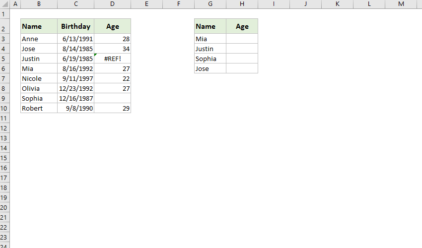
Normally if error cells exist in a reference table, the Vlookup function will return the errors too. See the screen shot below. Some users may not want to show the errors in the new table, therefore, how to ignore errors of original reference table when applying Vlookup function in Excel? Here we recommend two methods to solve it quickly.

- Ignore errors when using VLOOKUP by modifying original reference table
- Ignore errors when using VLOOKUP by combining Vlookup and IF functions
- Ignore errors when using VLOOKUP by an amazing tool
Ignore errors when using VLOOKUP by modifying original reference table
This method will walk you through changing the original reference table and get a new column/table without error values, and then applying the Vlookup function in this new column/table in Excel.
1. Besides original reference table, insert a blank column and enter a column name for it.
In our case, I insert a blank column right to Age column, and enter the column name of Age (Ignore Error) in the Cell D1.
2. Now in the Cell D2 enter below formula, and then drag the Fill Handle to the range you need.
=IF(ISERROR(C2),"",C2)

Now in the new Age (Ignore Error) column, the error cells are replaced by blank.
3. Now go to the cell (Cell G2 in our case) where you will get the vlookup values, enter below formula, and drag the Fill Handle to the range you need.
=VLOOKUP(F2,$A$2:$D$9,4,FALSE)

Now you will see if it's error in the original reference table, the Vlookup Function will return blank.
Quickly apply the VLOOKUP function and ignore errors in Excel
The VLOOKUP function will return 0 if the matched value does not exist, or return #N/A error occurring by various reasons in Excel. To ignoring the VLOOKUP errors, you may need to modify the VLOOKUP formulas one by one manually. Here, with the Replace 0 or #N/A with Blank or a Specified Value feature of Kutools for Excel, you can easily avoid returning errors values.
Kutools for Excel - Supercharge Excel with over 300 essential tools. Enjoy a full-featured 30-day FREE trial with no credit card required! Get It Now
Ignore errors when using VLOOKUP by combining Vlookup and IF functions
Sometimes, you may not want to modify the original reference table, therefore, combining the Vlookup function, IF function, and ISERROR function can help you check whether the vlookup returns errors and ignore these errors with ease.
Go to a blank cell (in our case we go to the Cell G2), enter the below formula, and then drag the Fill Handle to the range you need.
=IF(ISERROR(VLOOKUP(F2,$A$2:$C $9,3,FALSE)),"",VLOOKUP(F2,$A$2:$C $9,3,FALSE))

In above formula:
- F2 is the cell containing content you want to match in the original reference table
- $A$2:$C $9 is the original reference table
- This formula will return blank if matched value is error in the original reference table.
 |
Formula is too complicated to remember? Save the formula as an Auto Text entry for reusing with only one click in future! Read more… Free trial |
Ignore errors when using VLOOKUP by an amazing tool
If you have installed Kutools for Excel, you can apply its Replace 0 or #N/A with Blank or a Specified Value to ignore errors when applying the VLOOKUP function in Excel. Please do as follows:
Kutools for Excel- Includes more than 300 handy tools for Excel. Full feature free trial 30-day, no credit card required! Get It Now
1. Click Kutools > Super LOOKUP > Replace 0 or #N/A with Blank or a Specified Value to enable this feature.

2. In the popping out dialog, please do as follows:

(1) In the Lookup Values box, please select the range containing the lookup values.
(2) In the Output Range box, please select the destination range you will place the return values.
(3) Choose how to handle the return errors. If you want to not show errors, please tick the Replace 0 or #N/A error value with empty option; and if you want to mark the errors with text, please tick the Replace 0 or #N/A error value with a specified value option, and type in the specified text into below box;
(4) In the Data range box, please select the lookup table;
(5) In the Key column box, please select the specified column containing the lookup values;
(6) In the Return column box, please select the specified column containing the matched values.
3. Click the OK button.
Now you will see values matched with the lookup values are found out and placed in the destination range, and errors are placed with blank or the specified text too.

Related articles:
Best Office Productivity Tools
Supercharge Your Excel Skills with Kutools for Excel, and Experience Efficiency Like Never Before. Kutools for Excel Offers Over 300 Advanced Features to Boost Productivity and Save Time. Click Here to Get The Feature You Need The Most...
")
Office Tab Brings Tabbed interface to Office, and Make Your Work Much Easier
- Enable tabbed editing and reading in Word, Excel, PowerPoint, Publisher, Access, Visio and Project.
- Open and create multiple documents in new tabs of the same window, rather than in new windows.
- Increases your productivity by 50%, and reduces hundreds of mouse clicks for you every day!
")