How to apply conditional formatting based on VLOOKUP in Excel?

Suppose you are maintaining a list of student scores for the current and a previous semester, and you want to quickly identify which students have improved. In this scenario, you want to compare each student’s score in the current term with their result from the previous term and visually highlight those who performed better.

To highlight rows in the Score worksheet if a student's current score is higher than their score in the last semester, you can use VLOOKUP inside a conditional formatting rule. This approach is practical in academic performance monitoring, project milestone tracking, or any repeated-measure data analysis where comparison is necessary.

1. In the Score worksheet, select the range of student scores you want to evaluate (excluding headers; in this example, select B3:C26). Go to the Home tab, click Conditional Formatting, and select New Rule.

2. In the New Formatting Rule dialog, do the following:

1. Select Use a formula to determine which cells to format.
2. Enter the following formula in the Format values where this formula is true box:

   =VLOOKUP($B3,'Score of Last Semester'!$B$2:$C$26,2,FALSE) < Score!$C3

3. Click the Format button to choose your preferred formatting.

Note: In this formula,

• $B3 refers to the first student’s name in the Score sheet. When applying conditional formatting to multiple rows, Excel automatically adjusts this reference for each row.
• 'Score of Last Semester'!$B$2:$C$26 defines the lookup range for the previous semester's scores. Adjust the range as needed if your list is longer or starts/stops at different rows.
• 2 specifies that the values to retrieve from the lookup range are in its second column.
• Score!$C3 points to the current student's score in the worksheet being formatted.

3. In the Format Cells dialog, navigate to the Fill tab, choose a highlight color, then confirm with OK > OK to apply and exit the dialogs.

Once applied, the formatting will automatically highlight each student's row if the current semester's score is greater than the previous one, making it easy to spot positive trends at a glance.

If you notice that some rows are not being highlighted as expected, check that both sheets use matching names (no extra spaces/inconsistent spelling), and that your referenced ranges include all the necessary data. If VLOOKUP does not find a match, it will return an error, so ensuring consistent data layouts is essential for accurate results.

You might want to visually identify whether items in a list exist in another sheet—for example, flagging participants of a winners’ list who are also present in a master roster. Conditional formatting with VLOOKUP allows for real-time highlighting of matched or unmatched items, which is valuable in many event or participant management scenarios.

Note: Drag the y scroll bar to view above picture.

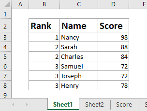
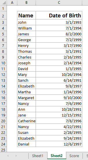
For this use case, you might have a winner list on Sheet1 and a full student roster on Sheet2. To highlight names in the winner list that are also present in the roster, proceed as follows:

1. Select the names in the winner list (excluding headers), then go to Home > Conditional Formatting > New Rule.

2. In the New Formatting Rule dialog, do the following:

1. In Select a Rule Type, choose Use a formula to determine which cells to format.
2. Enter the following formula in the Format values where this formula is true box:

   =NOT(ISNA(VLOOKUP($C3,Sheet2!$B$2:$C$24,1,FALSE)))

3. Click the Format button to set the highlighting style.

Note:

• $C3 refers to the first name in the winner list; ensure your selection matches your actual data's layout.
• Sheet2!$B$2:$C$24 is the lookup table containing the comprehensive student roster. Adjust the range as needed to fit your sheet.
• 1 indicates that VLOOKUP will search in the first column of the specified range.

If you need to highlight names from the winner list that are not found in the student roster, use the opposite formula:

=ISNA(VLOOKUP($C3,Sheet2!$B$2:$C$24,1,FALSE))

3. In the Format Cells dialog, go to the Fill tab, choose your preferred background color, then click OK > OK to finish.

After applying the rule, all names that satisfy your match or mismatch criteria will be highlighted automatically. This makes error checking, participant validation, or list reconciliation much more efficient.

Tip: If you encounter unexpected results, double-check your lookup ranges for extra spaces or inconsistent values that could interfere with VLOOKUP’s exact match logic. Consider using the TRIM function in helper columns to standardize your data if necessary.

If you have Kutools for Excel installed, you gain additional flexibility and ease for comparing lists and applying conditional formatting. The Select Same & Different Cells feature allows users to highlight matched or unmatched values with just a few clicks, minimizing the risk of errors common with manual formula entry.

Kutools for Excel includes more than300 practical tools for Excel, providing robust support for data comparison and formatting tasks. This is especially beneficial for those who regularly process extensive lists or diverse datasets. You can try the full feature set free for60 days with no credit card required.

1. Click Kutools > Select > Select Same & Different Cells to launch the tool.

2. In the Select Same & Different Cells dialog, configure your settings as follows:

1. In the Find Values in box, select the Name column of the winner list.
2. In the According to box, select the Name column of the student roster.
3. If your data contains headers, you can check the My data has headers option based on your needs.
4. Under Based on, choose Each Row for row-by-row comparison.
5. In the Find section, select either Same values or Different Values based on whether you want to highlight matches or discrepancies.
6. Check Fill backcolor and select a desired color for highlighting.
7. If you want to highlight the entire row, select Select entire rows.

3. Click OK to execute the operation. The tool will highlight and select the rows with matching (or different) values immediately. Additionally, a dialog box displays the count of selected rows, helping you quickly evaluate comparison results.

This method is most advantageous when working with long lists, as it eliminates the manual work of writing and troubleshooting formulas. Also, the visual feedback and summary dialog reduce guesswork and potential errors.