How to highlight the odd or even months in Excel?
Highlighting odd or even months in Excel can help make your data more visually organized and easier to analyze, especially when working with large datasets. Whether you’re tracking sales trends, project timelines, or attendance records, this formatting trick can quickly draw attention to specific months. In this article, we’ll explore different methods to highlight odd or even months in Excel.

Highlight the odd or even months with Conditional Formatting
In Excel, the powerful Conditional Formatting feature can help you to achieve this task quickly and easily, please do as this:
1. Select the data range that you want to highlight the odd or even months, and then click "Home" > "Conditional Formatting" > "New Rule", see screenshot:

2. In then popped out "New Formatting Rule" dialog box, do the following operations:
- Click "Use a formula to determine which cells to format" from the "Select a Rule Type" list box;
- Then, type this formula: =MOD(MONTH($D2),2) into the Format values where this formula is true text box;
- Finally, click "Format" button.

3. In the "Format Cells" dialog box, under the "Fill" tab, select one color you like to fill the rows, see screenshot:

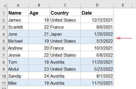
4. And then, click OK > OK to close the dialog boxes. And now, the rows contain the odd months are filled with the color you specified at once, see screenshot:

Highlight the odd or even months with Kutools AI
While Excel’s built-in Conditional Formatting can handle this task with formulas, Kutools AI provides a faster, more intuitive solution that simplifies the process, especially for those without advanced formula knowledge. In this section, we’ll guide you step-by-step on how to use Kutools AI to highlight odd or even months in your Excel effortlessly.
After installing Kutools For Excel, please click "Kutools" > "AI Aide" to open the "Kutools AI Aide" pane.
- Select the data range that you want to remove text within parentheses;
- Then, type the requirement in the chat box: such as:
● Highlight odd months:
Highlight the rows with odd months in the selection with a light blue color
● Highlight even months:
Highlight the rows with even months in the selection with a light blue color - And then, press Enter key or click the "Send" button. Kutools AI will analyze the question, after finishing, please click "Execute" button to get the result.
Highlighting odd or even months in Excel can be done effectively using Conditional Formatting and Kutools, by applying these methods, you can make your data more visually organized and easier to interpret, saving time and improving accuracy in your analysis. If you're interested in exploring more Excel tips and tricks, our website offers thousands of tutorials.
Best Office Productivity Tools
Supercharge Your Excel Skills with Kutools for Excel, and Experience Efficiency Like Never Before. Kutools for Excel Offers Over 300 Advanced Features to Boost Productivity and Save Time. Click Here to Get The Feature You Need The Most...
Office Tab Brings Tabbed interface to Office, and Make Your Work Much Easier
- Enable tabbed editing and reading in Word, Excel, PowerPoint, Publisher, Access, Visio and Project.
- Open and create multiple documents in new tabs of the same window, rather than in new windows.
- Increases your productivity by 50%, and reduces hundreds of mouse clicks for you every day!
All Kutools add-ins. One installer
Kutools for Office suite bundles add-ins for Excel, Word, Outlook & PowerPoint plus Office Tab Pro, which is ideal for teams working across Office apps.
- All-in-one suite — Excel, Word, Outlook & PowerPoint add-ins + Office Tab Pro
- One installer, one license — set up in minutes (MSI-ready)
- Works better together — streamlined productivity across Office apps
- 30-day full-featured trial — no registration, no credit card
- Best value — save vs buying individual add-in