Goal Seek, a part of Excel's what-if analysis toolkit, is a powerful feature used for backward calculations. Essentially, if you know the desired outcome of a formula but are not sure what input value will produce this result, you can use Goal Seek to find it. Whether you're a financial analyst, a student, or a business owner, understanding how to use Goal Seek can significantly streamline your problem-solving process. In this guide, we will explore what Goal Seek is, how to access it, and demonstrate its practical applications through various examples, ranging from adjusting loan payment plans to calculating the minimum scores for exams and more.

• Example 1: Adjusting a loan payment plan
• Example 2: Determining the minimum score for passing the exam
• Example 3: Calculating required votes for election victory
• Example 4: Achieving target profit in a business

What is Goal Seek in Excel?

Goal Seek is an integral feature of Microsoft Excel, part of its suite of what-if analysis tools. It enables users to perform reverse calculations – instead of calculating the result of given inputs, you specify the desired result and Excel adjusts an input value to achieve that goal. This functionality is particularly useful in scenarios where you need to find the input value that will produce a specific outcome.

• Single variable adjustment:
  Goal Seek can only change one input cell value at a time.
• Requires a formula:
  When applying the Goal Seek feature, the target cell must contain a formula.
• Maintain the integrity of the formula:
  Goal Seek does not alter the formula in the target cell; it changes the value in the input cell that the formula depends on.

Accessing Goal Seek in Excel

To access the Goal Seek feature, go to the Data tab, click What-If Analysis > Goal Seek. See screenshot:

Then the Goal Seek dialog box pops up. Here's an explanation of the three options in Excel's Goal Seek dialog box:

• Set Cell: The target cell that contains the formula you want to achieve. This cell must contain a formula, and Goal Seek will adjust the values in another related cell to make this cell's value reach your set goal.
• To Value: The target value you want the "Set Cell" to reach.
• By Changing Cell: The input cell that you want Goal Seek to adjust. The value in this cell will be changed to ensure the value in the "Set Cell" meets the "To Value" target.
  
  

In the next section, we'll explore how to utilize Excel's Goal Seek feature through detailed examples.

Using Goal Seek with examples

In this section, we'll walk through four common examples that demonstrate the usefulness of Goal Seek. These examples will range from personal finance adjustments to strategic business decisions, offering insights into how this tool can be applied in various real-world scenarios. Each example is designed to give you a clearer understanding of how to effectively use Goal Seek to solve different types of problems.

Example 1: Adjusting a Loan Payment Plan

Scenario: A person plans to take out a loan of $20,000 and aims to repay it in 5 years at an annual interest rate of 5%. The required monthly repayment is $377.42. Later, he realizes that he can increase his monthly repayment by $500. Given that the total loan amount and the annual interest rate remain the same, how many years will it now take to pay off the loan?

As the following table shown:

• B1 contains the loan amount $20000.
• B2 contains the loan term 5 (years).
• B3 contains the annual interest rate 5%.
• B5 contains the monthly payment that is calculated by formula =PMT(B3/12,B2*12,B1).
  
  

Here I will show you how to use the Goal Seek feature to accomplish this task.

Step 1: Activate the Goal Seek feature

Go to the Data tab, click What-If Analysis > Goal Seek.

Step 2: Configure the Goal Seek settings

1. In the Set cell box, select the formula B5.
2. In the To value box, input the monthly scheduled repayment amount -500 (a negative number represents a payment).
3. In the By changing cell box, select the cell B2 you want to adjust.
4. Click OK.
   
   

Result

The Goal Seek Status dialog box will then appear, showing that a solution has been found. At the same time, the value in cell B2 that you specified in the “By changing cell” box will be replaced with the new value, and the formula cell will get the target value based on the variable change. Click OK to apply the changes

Now, it will take him about 3.7 years to pay off the loan.

Example 2: Determining the minimum score for passing the exam

Scenario: A student needs to take 5 exams, each with equal weight. To pass, the student must achieve an average score of 70% across all exams. Having completed the first 4 exams and knowing their scores, the student now needs to calculate the minimum score required on the fifth exam to ensure the overall average reaches or exceeds 70%.

As shown in the screenshot below:

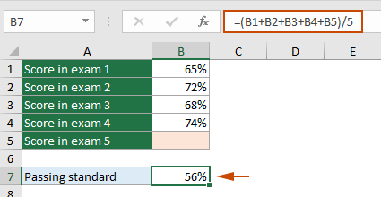
• B1 contains the score of the first exam.
• B2 contains the score of the second exam.
• B3 contains the score of the third exam.
• B4 contains the score of the fourth exam.
• B5 will contain the score of the fifth exam.
• B7 is the passing average score that is calculated by formula =(B1+B2+B3+B4+B5)/5.
  
  

To achieve this goal, you can apply the Goal Seek feature as follows:

Step 1: Activate the Goal Seek feature

Go to the Data tab, click What-If Analysis > Goal Seek.

Step 2: Configure the Goal Seek settings

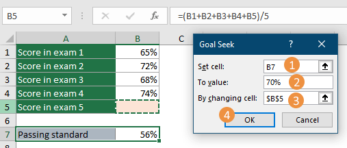
1. In the Set cell box, select the formula cell B7.
2. In the To value box, enter the passing average score 70%.
3. In the By changing cell box, select the cell (B5) you want to adjust.
4. Click OK.
   
   

Result

The Goal Seek Status dialog box will then appear, showing that a solution has been found. At the same time, the cell B7 that you specified in the “By changing cell” box will be automatically entered with a matching value, and the formula cell will get the target value based on the variable change. Click OK to sccept the solution.

So, to achieve the required overall average and pass all exams, the student needs to score at least 71% on the last exam.

Example 3: Calculating Required Votes for Election Victory

Scenario: In an election, a candidate needs to calculate the minimum number of votes required to secure a majority. With the total number of votes cast known, what is the minimum number of votes the candidate must receive to achieve more than 50% and win?

As shown in the screenshot below:

• Cell B2 contains the total number of votes cast in the election.
• Cell B3 shows the current number of votes received by the candidate.
• Cell B4 contains the desired majority (%) of votes the candidate aims to achieve, which is calculated by formula =B2/B1.
  
  

To achieve this goal, you can apply the Goal Seek feature as follows:

Step 1: Activate the Goal Seek feature

Go to the Data tab, click What-If Analysis > Goal Seek.

Step 2: Configure the Goal Seek settings

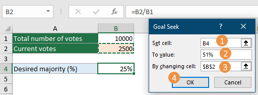
1. In the Set cell box, select the formula cell B4.
2. In the To value box, enter the desired percentage of majority votes. In this case, to win the election, the candidate must obtain more than half (i.e., over 50%) of the total valid votes, so I enter 51%.
3. In the By changing cell box, select the cell (B2) you want to adjust.
4. Click OK.
   
   

Result

The Goal Seek Status dialog box will then appear, showing that a solution has been found. At the same time, the cell B2 that you specified in the “By changing cell” box will be automatically replaced with the new value, and the formula cell will get the target value based on the variable change. Click OK to apply the changes.

So, the candidate needs at least 5100 votes to win the election.

Example 4: Achieving Target Profit in a Business

Scenario: A company aims to achieve a specific profit target of $150,000 for the current year. Considering both fixed and variable costs, they need to determine the necessary sales revenue. How many units of sales are required to reach this profit goal?

As shown in the screenshot below:

• B1 contains the fixed costs.
• B2 contains the variable costs per unit.
• B3 contains the price per unit.
• B4 contains the units sold.
• B6 is the total revenue, which is calculated by formula =B3*B4.
• B7 is the total cost, which is calculated by formula =B1+(B2*B4).
• B9 is the current profit on sales, which is calculated by formula =B6-B7.
  
  

To get the total units of sales based on target profit, you can apply the Goal Seek feature as follows.

Step 1: Activate the Goal Seek feature

Go to the Data tab, click What-If Analysis > Goal Seek.

Step 2: Configure the Goal Seek settings

1. In the Set cell box, select the formula cell that returns the profit. Here is cell B9.
2. In the To value box, enter the target profit 150000.
3. In the By changing cell box, select the cell (B4) you want to adjust.
4. Click OK.
   
   

Result

The Goal Seek Status dialog box will then appear, showing that a solution has been found. At the same time, the cell B4 that you specified in the "By changing cell" box will be automatically replaced with a new value, and the formula cell will get the target value based on the variable change. Click OK to accept the changes.

As a result, the company needs to sell at least 6666 units to make its target profit of $150,000.

Common issues and solutions for Goal Seek

This section lists some common issues and corresponding solutions for Goal Seek.

1. Goal Seek Cannot Find a Solution

• Reason: This typically happens when the target value is not achievable with any possible input value, or if the initial guess is too far from any potential solution.
• Solution: Adjust the target value to ensure it is within a feasible range. Also, try different initial guesses closer to the expected solution. Ensure that the formula in the "Set Cell" is correct and can logically produce the desired "To Value".

2. Slow Calculation Speed

• Reason: Goal Seek can be slow with large datasets, complex formulas, or when the initial guess is far from the solution, requiring more iterations.
• Solution: Simplify the formulas where possible and reduce the data size. Ensure that the initial guess is as close as possible to the expected solution to reduce the number of iterations needed.

3. Accuracy Issues

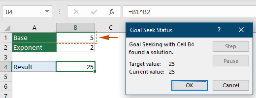
• Reason: When using Goal seek, you may notice that sometimes Excel will say it found a solution, but it's not exactly what you want - close but not close enough. Goal Seek may not always provide a highly accurate result due to Excel's calculation precision and rounding.
  
  For example, to calculate a specific exponentiation of a number and use Goal Seek to find the base that achieves a desired result. Here I will change the input value in cell A1 (Base) so that cell A3 (result of exponentiation) matches the target result of 25.
  
  As you can see in the screenshot below, Goal Seek provides an approximate value rather than the exact root.
  
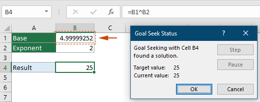
• Solution: Increase the number of decimal places shown in Excel’s calculation options for more accuracy then rerun the Goal Seek feature. Please do as follows.
  
  1. Click File > Options to open the Excel Options window.
  2. Select Formulas in the left pane, and in the Calculation options section, increase the number of decimal places in the Maximum Change box. Here I change 0.001 to 0.000000001 and click OK.
     
  3. Re-run the Goal Seek and you will get the exact root as shown in the screenshot below.
     

4. Limitations and Alternative Methods

• Reason: Goal Seek can adjust only one input value and might not be suitable for equations requiring simultaneous adjustments of multiple variables.
• Solution: For scenarios needing adjustments of multiple variables, use Excel's Solver, which is more powerful and allows for constraints setting.

Goal Seek is a powerful tool for performing reverse calculations, sparing you from the tedious task of manually testing different values to approximate your target. Equipped with the insights from this article, you can now apply Goal Seek with confidence, propelling your data analysis and efficiency to new heights. For those eager to delve deeper into Excel's capabilities, our website boasts a wealth of tutorials. Discover more Excel tips and tricks here.