In the realm of Excel, various symbols and operators play pivotal roles in formula creation and data manipulation. Among these, the ampersand (&) symbol stands out for its ability to concatenate, or link together, multiple strings of text. Understanding its function is key to mastering Excel's powerful data handling capabilities.

The Essence of & in Excel
Basic and Practical Uses of “&” in Excel

• Combining Names
• Creating Email Addresses
• Concatenating Multiple Cells

Advanced Uses of "&" in Excel

• Merging Text with Formula
  
• Dynamic Formulas (with IF Function)
• Conditional Formatting with Text Concatenation
• Creating Complex Strings

The Essence of & in Excel

At its core, the & operator in Excel is a concatenation tool. It's used to join two or more text strings into one continuous string. This operator becomes invaluable when you need to merge data from different cells or combine text and numbers for clearer data representation. Whether it's for simple tasks like merging names or for complex operations involving dynamic data structures, understanding and utilizing the & operator is a skill that can greatly enhance your proficiency with Excel. It's a small symbol with big possibilities, transforming the way you interact with data.

Basic Uses of “&” in Excel

The ampersand (&) sign is primarily utilized to merge two or more cells into a single entity. This is commonly applied to actions such as joining a person's first name with their last name, generating email addresses from names, amalgamating text and numerical values, and concatenating various cells to form a unified content.

Combining Names (Concatenate Two Cells)

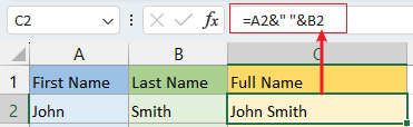
Scenario: You have a list of first and last names in separate columns (column A and column B) and you want to combine them.

Formula: Select a blank cell (C2) and type one of below formulas to combine the first names and last names. Then press Enter key to get the first combination.

Combine first and last name without any separator

=A2&B2 

Combine first and last name with a space

=A2&" "&B2 

Combine without separator	Combine with space as separator

Then drag auto fill handle down to get all full names.

Combine without separator	Combine with space as separator

Creating Email Addresses (Concatenate A Fixed Text with Cell Reference)

Scenario: From a list of employee names (A2:A6), you need to generate email addresses.

Formula: Select a blank cell (B2) and type below formula to combine the names and company email domain. Then press Enter key to get the first combination.

=A2&"@company.com"

Then drag auto fill handle down to get all email addresses.

Concatenating Multiple Cells (Merging Three or More Cells)

Scenario: Creating a comma-separated list from multiple cells. (Combine each row cells from column A to column C.)

Formula: Select a blank cell (D2) and type below formula to combine cells A2, B2 and C2 with commas. Then press Enter key to get the first combination.

=A2&", "&B2&", "&C2

Then drag auto fill handle down to get all combinations.

Advanced Uses of "&" in Excel

The ampersand (&) in Excel, while simple in its basic function of text concatenation, can be a powerful tool in more complex and dynamic scenarios. Here's a deeper look into its advanced applications, particularly in dynamic functions and conditional formatting.

Merging Text with Formula

Scenario: From a table of data, you want to get the total of each column and add a descriptive text before each text.

Formula: Select a blank cell (A7) and type below formula to total A2:A6 and add a descriptive text before the total. Then press Enter key to get the first combination.

="Total sales: "&SUM(A2:A6)

Then drag auto fill handle right to get totals for each column.

Dynamic Formulas (with IF Function)

Scenario: Suppose you're preparing a report and need to include a dynamic message that changes based on data values. For example, you have a sales target column (B) and an actual sales column (C). and you want to create a status message in column D (display "target achieved" if the sale is equal to or greater than target, display "target missed" if the sale is less than the target).

Formula: Select a blank cell (D2) and type below formula. Then press Enter key to get the first combination.

=IF(C2 >= B2, "Target Achieved: "&C2, "Target Missed: "&C2)

Then drag auto fill handle down to get status for each row.

Conditional Formatting with Text Concatenation

Scenario: Highlighting cells with a specific status message that includes data from the cell itself. For example, a list of project names and their statuses in two columns (column A and B). You want to use conditional formatting to highlight projects with delayed status.

Apply Conditional Formatting: Select two column ranges (A2:B6), click Home > Conditional Formatting > New Rule.

Formula: Choose Use a formula to determine which cells to format, then copy below formula to the Format values where this formula is true textbox.

=ISNUMBER(SEARCH("Delayed", A2 & B2))

Format cells: Click Format button to open the Format Cells dialog, choose one color to highlight the row contains “Delayed” under Fill tab. Click OK > OK to close the dialogs.

Result:

Creating Complex Strings

Scenario: Building detailed descriptions or messages in a financial report. For example, column A contains products and column B to D containis the related sales for quarter 1. Now you want to create a descriptive text string for each total sales in quarter 1 like "the total sales of AA-1 for this quarter is $1,879.21".

Formula: Select a blank cell (E2) and type below formula. Then press Enter key to get the first combination.

="The total sales of " & A2 & " for this quarter is: $" & TEXT(SUM(B2:D2), "#,##0.00")

Then drag auto fill handle down to get all combinations.

The versatility of the & operator extends far beyond simple text merging. Its ability to integrate within dynamic formulas, enhance conditional formatting, and construct complex, informative strings, makes it an indispensable tool in advanced Excel data manipulation and presentation. These examples illustrate just a few of the ways & can be used to bring more sophistication and adaptability to your Excel tasks.

For more game-changing Excel strategies that can elevate your data management, explore further here..