When you have a complex formula dependent on multiple variables and want to understand how changing those inputs impacts the results efficiently, a What-If analysis data table in Excel is a powerful tool. It allows you to see all possible outcomes with a quick glance. Here's a step-by-step guide on how to create a data table in Excel. Additionally, we'll discuss some key points for using data tables effectively and demonstrate other operations such as deleting, editing, and recalculating data tables.

What is data table in Excel?

Create one-variable data table

• Column-oriented data table
• Row-oriented data table
• Multiple formulas for one-variable data table

Create two-variable data table

Key points using the data tables

Other operations for using data tables

• Delete a data table
• Edit data table result
• Recalculate data table manually

What is data table in Excel?

In Excel, a data table is one of the What-If Analysis tools that allows you to experiment with different input values for formulas and observe the changes in the formula's output. This tool is incredibly useful for exploring various scenarios and conducting sensitivity analyses, especially when a formula is dependent on multiple variables.

There are two types of data tables in Excel:

One-Variable Data Table: This allows you to analyze how different values of one variable will impact a formula. You can set up a one-variable data table in either a row-oriented or column-oriented format, depending on whether you want to vary your input across a row or down a column.

Two-Variable Data Table: This type allows you to see the impact of changing two different variables on a formula's outcome. In a two-variable data table, you vary the values along both a row and a column.

Create one-variable data table

Creating a one-variable data table in Excel is a valuable skill for analyzing how changes in a single input can impact various outcomes. This section will guide you through the process of creating column-oriented, row-oriented, and multiple-formula one-variable data tables.

Amazing! Using Efficient Tabs in Excel Like Chrome, Edge, Firefox and Safari!
Save 50% of your time, and reduce thousands of mouse clicks for you every day!

---

Column-oriented data table

A column-oriented data table is useful when you want to test how different values of a single variable impact a formula's output, with the variable values listed down a column. Let's consider a simple financial example:

Suppose you are considering a loan of $50,000, which you plan to repay over a span of 3 years (equivalent to 36 months). In order to evaluate what monthly payment would be affordable based on your salary, you're interested in exploring how various interest rates would affect the amount you need to pay each month.

Step 1: Set up the base formula

To calculate the payment, here, I will set the interest as 5%. In a cell B4, enter the PMT formula, it calculates the monthly payment based on the interest rate, number of periods, and loan amount. See screenshot:

= -PMT($B$1/12, $B$2*12, $B$3)

Step 2: List the interest rates in a column

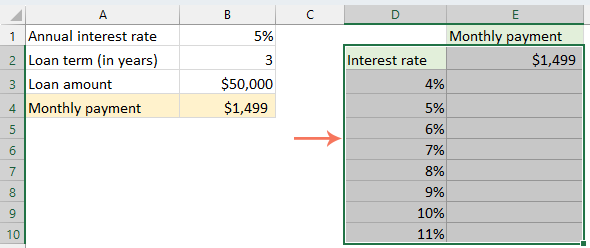
In a column, list the different interest rates you want to test. For example, list values from 4% to 11% in increments of 1% in a column, and leave at least one blank column to the right for the outcomes. See screenshot:

Step 3: Create the data table

1. In the cell E2, enter this formula: =B4.
   
   Note: B4 is the cell where your main formula is located, this is the formula whose results you want to see change as you vary the interest rate.
   
2. Select the range that includes your formula, list of interest rates and adjacent cells for the results (e.g., select D2 to E10). See screenshot:
   
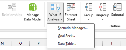
3. Go to the ribbon, click on the Data tab, then click What-If Analysis > Data Table, see screenshot:
   
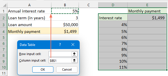
4. In the Data Table dialog box, click in the Column Input cell box (since we're using a column for input values), and select the variable cell referenced in your formula. In this example, we select B1 that contains the interest rate. At last, click OK button, see screenshot:
   
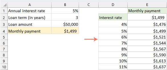
5. Excel will automatically fill the empty cells adjacent to each of your variable values (different interest rates) with the corresponding outcomes. See screenshot:
   
6. Apply the desired number format to the results (Currency) to your need. Now, the column-oriented data table is created successfully, and you can swiftly peruse the results to evaluate which monthly payment amounts would be affordable for you when the interest rate changes. See screenshot:
   

Row-oriented data table

Creating a row-oriented data table in Excel involves arranging your data so that the variable values are listed across a row rather than down a column. Taking the above example as a reference, let's proceed with the steps to complete the creation of row-oriented data table in Excel.

Step 1: List the interest rates in a row

Place the variable values (interest rates) in a row, ensuring there is at least one empty column to the left for the formula and one empty row below for the results, see screenshot:

Step 2: Create the data table

1. In the cell A9, enter this formula: =B4.
   
2. Select the range that includes your formula, list of interest rates and adjacent cells for the results (e.g., select A8 to I9). Then, click Data > What-If Analysis > Data Table.
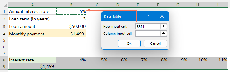
3. In the Data Table dialog box, click in the Row input cell box (since we're using a row for input values), and select the variable cell referenced in your formula. In this example, we select B1 that contains the interest rate. At last, click OK button, see screenshot:
   
4. Apply the desired number format to the results (Currency) to your need. Now, the row-oriented data table is created, see screenshot:
   

Multiple formulas for one-variable data table

Creating a one-variable data table with multiple formulas in Excel allows you to see how changing a single input affects several different formulas at once. In the above example, what if you want to see the change in interest rates on both the repayments and total interest? Here’s how to set it up:

Step 1: Add a new formula to calculate the total interest

In cell B5, enter the following formula to calculate the total interest:

=B4*B2*12-B3

Step 2: Arrange the data table's source data

In a column, list the different interest rates you want to test, and leave at least two blank columns to the right for the outcomes. See screenshot:

Step 3: Create the data table:

1. In cell E2, enter this formula: =B4 to create a reference to the repayment calculation in the original data.
2. In cell F2, enter this formula: =B5 to create a reference to the total interest in the original data.
   
3. Select the range that includes your formulas, list of interest rates and adjacent cells for the result (e.g., select D2 to F10). Then, click Data > What-If Analysis > Data Table.
4. In the Data Table dialog box, click in the Column input cell box (since we're using a column for input values), and select the variable cell referenced in your formula. In this example, we select B1 that contains the interest rate. At last, click OK button, see screenshot:
   
5. Apply the desired number format to the results (Currency) to your need. And you can see the results for each formula based on the varying variable values.
   

Create two-variable data table

A two-variable data table in Excel displays the impact of different combinations of two sets of variable values on a formula's outcome, demonstrating how alterations in two inputs of a formula simultaneously affect its result.

Here, I have drawn a simple sketch to help you better understand the appearance and structure of a two-variable data table.

Building on the example to create one-variable data table, let's now go on learning how to create a two-variable data table in Excel.

In the below data set, we have the interest rate, loan term and loan amount, and have calculated the monthly payment by using this formula: =-PMT($B$1/12, $B$2*12, $B$3) as well. Here, we will focus on two key variables from our data: interest rate and loan amount, to observe how changes in both these factors simultaneously affect the repayment amounts.

Step 1: Set up the two changing variables

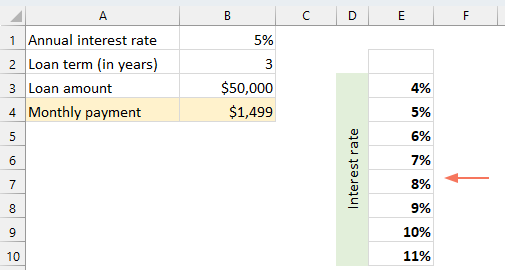
1. In a column, list the different interest rates you want to test. see screenshot:
   
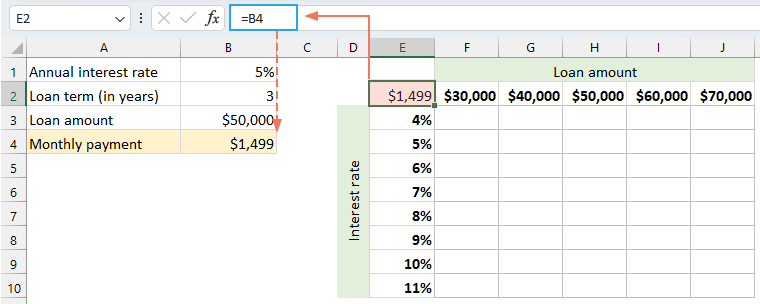
2. In a row, enter the different loan amount values just above the column values (starting from one cell to the right of the formula cell), see screenshot:
   

Step 2: Create the data table

1. Place your formula at the intersection of the row and the column where you listed the variable values. In this case, I will enter this formula: =B4 into cell E2. See screenshot:
   
2. Select the range that includes your loan amounts, interest rates, the formula cell, and the cells where the results will be displayed.
   
3. Then, click Data > What-If Analysis > Data Table. In the Data Table dialog box:
   • In the Row input cell box, select the cell reference to the input cell for the variable values in the row (in this example, B3 contains the loan amount).
   • In the Column input cell box, select the cell reference to the input cell for the variable values in the column (B1 contains the interest rate).
   • And then, click OK Button.
     
4. Now, Excel will fill in the data table with the results for each combination of loan amount and interest rate. It provides a direct view of how different combinations of loan amounts and interest rates affect the monthly payment, making it a valuable tool for financial planning and analysis.
   
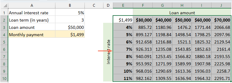
5. Finally, you should apply the desired number format to the results (Currency) to your need.
   

Key points using the data tables

• The newly created data table must be in the same worksheet as the original data.
• The output of the data table depends on the formula cell in the source data set, and any changes to this formula cell will automatically update the output.
• Once values have been calculated using the data table, they cannot be undone with Ctrl + Z. However, you can manually select all the values and delete them.
• The data table generates array formulas, so individual cells within the table cannot be altered or deleted.

Other operations for using data tables

Once you have created a data table, you might require additional operations to manage it effectively, including deleting the data table, modifying its results, and performing manual recalculations.

Delete a data table

Because the data table results are calculated with an array formula, you cannot delete an individual value from the data table. However, you can only delete the whole data table.

Select all the data table cells or only the cells with the results, and then press Delete key on keyboard.

Edit data table result

Indeed, it's not possible to edit individual cells within a data table directly, as they contain array formulas that Excel generates automatically.

To make changes, you would typically need to delete the existing data table and then create a new one with the desired modifications. This involves adjusting your base formula or the input values and then setting up the data table again to reflect these changes.

Recalculate data table manually

Normally, Excel recalculates all the formulas in all open workbooks every time a change is made. If a large data table containing numerous variable values and complex formulas is causing your Excel workbook to slow down.

To avoid Excel automatically performing calculations for all data tables each time a change is made in the workbook, you can switch the calculation mode from Automatic to Manual. Please do as follows:

Go to the Formulas tab, and then click Calculation Options > Automatic Except for Data Tables, see screenshot:

Once you modify this setting, when you recalculate your whole workbook, Excel will no longer automatically update the calculations in your data tables.

If you need to update your data table manually, just select the cells where the results (cells containing the TABLE() formulas) are displayed, and then press F9 key.

By following the steps outlined in this guide and keeping the key points in mind, you can efficiently utilize data tables for your data analysis needs. If you're interested in exploring more Excel tips and tricks, our website offers thousands of tutorials, please click here to access them. Thank you for reading, and we look forward to providing you with more helpful information in the future!