Excel IF function

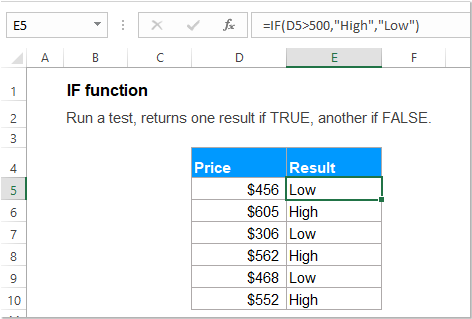
The IF function is one of simplest and most useful functions in Excel workbook. It performs a simple logical test which depending on the comparison result, and it returns one value if a result is TRUE, or another value if result is FALSE.

---

 Syntax:

The syntax for the IF function in Excel is:

---

 Arguments:

• logical_test: Required. It is the condition that you want to test.
• value_if_true: Optional. A specific value that you want returned if the logical_test result is TRUE.
• value_if_false: Optional. A value that you want returned if the logical_test result is FALSE.

---

 Return:

Test for a specific condition, returns the corresponding value that you supply for TRUE or FALSE.

---

 Examples:

Example 1: Using a simple IF function for numbers

For example, supposing, you want to test a list of values, if the value is greater than a specific value 100, a text “Good” is displayed, if not, a text “Bad” is returned.

Enter the below formula, and you will get the below result as you need.

---

Example 2: Using IF function for text values

Case 1: IF function for text values with case insensitive:

Here, I have a table with a list of Tasks and Completion Status, now, I want to know which tasks need to be go on, and which needn’t. When the text in Column C is completed, “No” will be displayed, otherwise, “Yes” will be returned.

Please apply the following formula, now, the cell will return “No” when text in column C is displayed as “completed”, no matter it is uppercase or lowercase; if other text in column C, “Yes” will be returned. See screenshot:

Case 2: IF function for text values with case sensitive:

To test the text values with case sensitive, you should combine the IF function with the EXACT function, please apply below formula, then only the text with the exact match will be recognized, and you will get the below result as you want:

Case 3: IF function for text values with partial match:

Sometimes, you need to check the cell values based on partial text, in this case, you should use the IF, ISNUMBER and SEARCH functions together.

For example, if you want to check the cells which contain the text “comp”, and then return the corresponding values, please apply the below formula. And you will get the result as below screenshot shown:

Notes:

• 1. The SEARCH function is applied for text with case insensitive, if you want to check the text with case sensitive, you should replace the SEARCH function with FIND function. Like this:=IF(ISNUMBER(FIND("comp",C2)), "No", "Yes")
• 2. The text values as parameters in the IF formulas, you must enclose them in "double quotes".

---

Example 3: Using IF function for date values

Case 1: IF function for dates to compare dates with a specific date:

If you want to compare dates to check if they are greater or less than a specific date, the IF function also can do you a favor. As the IF function cannot recognize a date format, you should combine a DATEVALUE function with it.

Please apply this formula, when the date is greater than 4/15/2019, a “Yes” will be returned, otherwise, the formula will return a “No” text, see screenshot:

Note: In the above formula, you can use the cell reference directly without using the DATEVALUE function as well. Like this: =IF(D4>$D$1, "Yes", "No").

Case 2: IF function for dates to check dates is greater or less than 30 days:

If you want to identify the dates which are greater or less than 30 days from current date, you can combine the TODAY function with the IF function.

Please enter this formula:

Identify the date older than 30 days: =IF(TODAY()-C4>30,"Older date","")

Identify the date greater than 30 days: =IF(C4-TODAY()>30, "Future date", "")

Note: If you would like to put the both results into one column, you need use a nested IF function as this:

---

Example 4: Using IF function with AND, OR function together

It is a common usage for us to combine the IF, AND, OR functions together in Excel.

Case 1: Using the IF function with AND functions to check if all conditions are true:

I want to check if all the conditions I set are met, such as: B4 is Red, C4 is Small and D4>200. If all conditions are TURE, mark the result as “Yes”; If either condition is FALSE, then return “No”.

Please apply this formula, and you will get the result as following screenshot shown:

Case 2: Using the IF function with OR functions to check any one of the conditions is true:

You can also use IF and OR functions to check if any one of the conditions is true, for example, I want to identify if the cell in column B contains the “Blue” or “Red” text, if any text in column B, Yes is displayed, otherwise, No is returned.

Here, you should apply this formula, and the below result will be shown:

Case 3: Using the IF function with AND and OR functions together:

This example, I will combine the IF function with both AND & OR functions at the same time. Supposing, you should check the following conditions:

• Condition 1: Column B = “Red” and Column D > 300;
• Condition 2: Column B = “Blue” and Column D > 300.

If either of the above conditions is met, a Match is returned, otherwise, No.

Please use this formula, and you will get the below result as you need:

---

Example 5: Using Nested IF function

IF function is used to test a condition and return one value if the condition is met and another value if it is not met. But, sometimes, you should need to check more than one condition at the same time and return different values, you can use Nested IF to solve this job.

A Nested IF statement which combines multiple IF conditions, it means putting an IF statement inside another IF statement and repeating that process multiple times.

The syntax for Nested IF function in Excel is:

Case 1: Nested IF function to check multiple conditions:

A classic use of the Nested IF function is to assign letter grade for each student based on their scores. For example, you have a table with students and their exam scores, now you want to classify the scores with the following conditions:

Please apply this formula, and you will get the below result, if the score is greater or equal to 90, the grade is “Excellent”, if the score is greater or equal to 80, the grade is “Good”, if the score is greater or equal to 60, the grade is “Medium”, otherwise, the grade is “Poor”.

Explanation of the above formula:

IF(check if C2>=90, if true - returns "Excellent", or else IF(check if C2>=80, if true - returns "Good", or else IF(check if C2>=60, if true - returns "Medium", if false - returns "Poor")))

Case 2: Nested IF function for calculating price based on quantity:

The Nested IF function also can be used to calculate the product price based on quantity.

For example, you want to provide customers a price break based on quantity, more quantity they purchase, more discount they will get as below screenshot shown.

As the total price equals quantity multiply the price, so you should multiply the specified quantity by the value returned by nested Ifs. Please use this formula:

Note: You can also use the cell references to replace the static price numbers, when the source data changing, you shouldn’t need to update the formula, please use this formula: =D2*IF(D2>=101, B6, IF(D2>=50, B5, IF(D2>=25, B4, IF( D2>=11, B3, IF(D2>=1, B2, "")))))

Tips: Using the IF function to construct a test, you can use the following logical operators:

Operator	Meaning	Example	Description
>	Greater than	=IF(A1>10, "OK",)	If the number in cell A1 is greater than 10, the formula returns "OK"; otherwise 0 is returned.
<	Less than	=IF(A1<10, "OK", "")	If the number in cell A1 is less than 10, the formula returns "OK"; otherwise an empty cell is returned.
>=	Greater than or equal to	=IF(A1>=10, "OK", "Bad")	If the number in cell A1 is greater than or equal to 10, it will return "OK"; otherwise, "Bad" is displayed.
<=	Less than or equal to	=IF(A1<=10, "OK", "No")	If the number in cell A1 is less than or equal to 10, it returns "OK"; otherwise, “No” is returned.
=	Equal to	=IF(A1=10, "OK", "No")	If the number in cell A1 is equal to 10, it returns "OK"; otherwise it displays "No".
<>	Not equal to	=IF(A1<>10, "No", "OK")	If the number in cell A1 is not equal to 10, the formula returns "No "; otherwise - "OK".