Excel ROW Function

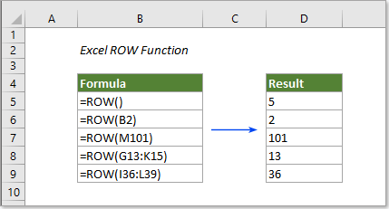
The Excel ROW function returns the row number of a reference.

Syntax

=ROW ([reference])

Arguments

Return value

The ROW function will return a number which representing the row of a reference.

Examples

The ROW function is very simple and easy to use in our Excel daily work. This section is going to show you some examples of ROW function to help you easily understand and use it in the future.

Example 1: The basic usage of ROW function in Excel

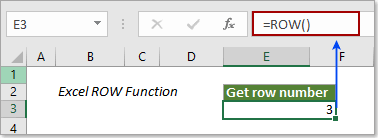
Select a cell and enter formula =ROW() into it will get the row number of this cell immediately.

As the below screenshot shown, copy the below formula into cell E3 will return the result as number 3.
=ROW()

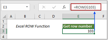
If specify a cell reference in the ROW function, such as =ROW(G103), it will return the row number 103 as below screenshot shown.

Example 2: Automatically number rows in Excel with ROW function

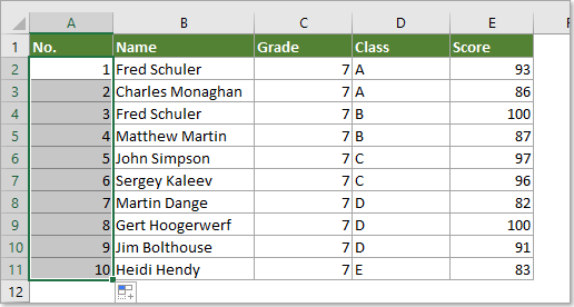
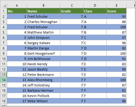
The ROW function can help to automatically number rows, and the created serial numbers will be updated automatically when adding or deleting rows from the range. See the below demo:

1. Supposing you want to start your serial numbers from 1 in cell A2, please select the cell and copy the below formula into it and press the Enter key.
=ROW()-1

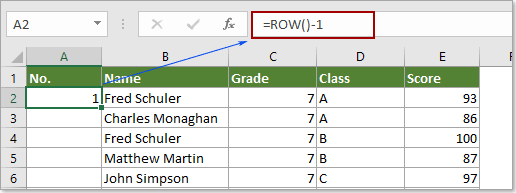
Note: If the beginning cell is A5, apply this formula =ROW()-4. Please subtract the row number above the current cell from where you are starting the serial number.

2. Keep selecting cell A2, drag the Fill Handle across the rows to create the series you need. See screenshot:

Example 3: highlight every other row (alternate rows) in Excel with ROW function

In this example, we explain how to shade every other row (alternate rows) in Excel by using the ROW function. Please do as follows.

1. Select the range you want to apply color to the alternate rows, click Conditional Formatting > New Rule under the Home tab. See screenshot:

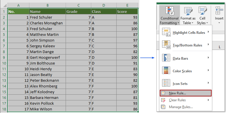
2. In the New Formatting Rule dialog box, you need to:

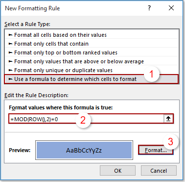
• 2.1) Select the Use a formula to determine which cells to format option in the Select a Rule Type box;
• 2.2) Enter formula =MOD(ROW(),2)=0 into the Format values where this formula is true box;
• 2.3) Click the Format button to specify a Fill color;
• 2.4) Click the OK button. See screenshot:

Note: The formula =MOD(ROW(),2)=0 means that all even rows in the selected range will be highlighted with certain fill color. If you want to shade all odd rows in the selected range, please change the 0 to 1 in the formula.

Then you can see all even rows in selected range are highlighted immediately.