Excel TAKE function
The TAKE function returns a specified number of contiguous rows or columns from the start or end of a given array.
Note: This function is only available in Excel for Microsoft 365 on the Insider channel.
Syntax
=TAKE(array, rows, [columns])
Arguments
Remarks
Return value
It returns a subset of a given array.
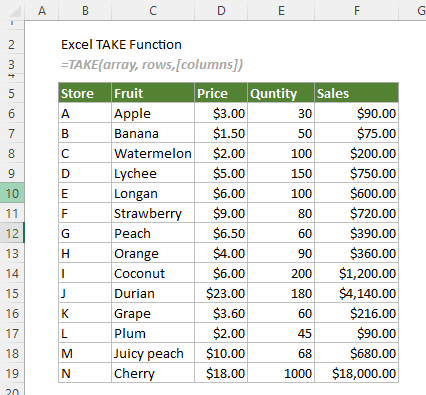
Example
Here we take the following sales table as an example to show you how to use the TAKE function to return a specified subset from it.
#Example1: Take the specified number of rows or columns only
For example, you want to take only the first three rows or columns from the sales table. You can apply one of the formulas below to get it done.
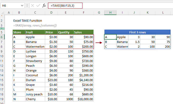
Take the specified number of rows only
To take a specified number of rows only, such as the first three rows, you need to ignore the columns argument.
Select a cell, say H6 in this case, enter the formula below and press the Enter key to get the specified subset.
=TAKE(B6:F19,3)
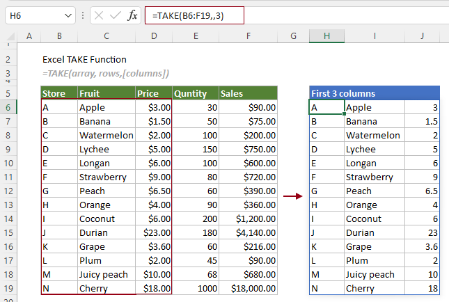
Take the specified number of columns only
To take a specified number of columns only, such as the first three columns, you need to leave the rows argument blank.
Select a cell, say H6 in this case, enter the formula below and press the Enter key to get the specified subset.
=TAKE(B6:F19,,3)
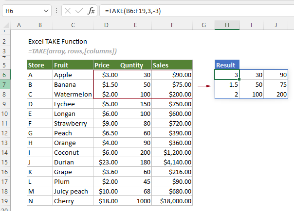
#Example2: Take specific rows or columns from the end of an array
In the examples above, you can see that the rows and columns are returned from the start of the array. That’s because you have specified a positive number for the rows or columns argument.
To take rows and columns from the end of an array, you need to specify a negative number for rows or columns argument.
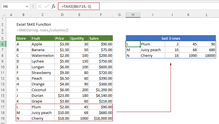
Take the last three rows
Select a cell, say H6 in this case, enter the formula below and press the Enter key to get the last three rows of the sales table.
=TAKE(B6:F19,-3)
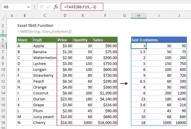
Take the last three columns
Select a cell, say H6 in this case, enter the formula below and press the Enter key to get the last three columns of the sales table.
=TAKE(B6:F19,,-3)
#Example3: Take the last 3 columns of the first two rows from an array
For example, you need to take the last 3 columns of the first two rows from an array, numbers should be provided for both the rows and columns. The formula is as follows:
=TAKE(B6:F19,2,-3)
The Best Office Productivity Tools
Kutools for Excel - Helps You To Stand Out From Crowd
Kutools for Excel Boasts Over 300 Features, Ensuring That What You Need is Just A Click Away...
Office Tab - Enable Tabbed Reading and Editing in Microsoft Office (include Excel)
- One second to switch between dozens of open documents!
- Reduce hundreds of mouse clicks for you every day, say goodbye to mouse hand.
- Increases your productivity by 50% when viewing and editing multiple documents.
- Brings Efficient Tabs to Office (include Excel), Just Like Chrome, Edge and Firefox.