How to hide zero data labels in chart in Excel?
When creating charts in Excel, adding data labels helps to clarify data points and provide viewers with direct access to values. However, when your charted data includes zeros, Excel will often display these zeros as data labels, potentially causing confusion or making the chart less visually appealing. In many business, academic, or reporting scenarios, it's common to prefer hiding these zero data labels so that only truly significant values are displayed in the chart.
Fortunately, Excel offers several practical methods to hide zero data labels, each suited to different needs and workflows. This tutorial summarizes popular approaches, including built-in formatting, formula-based methods, and even automation with VBA. Read on for step-by-step instructions and helpful tips to ensure your charts display only the data that matters.
- Hide zero data labels in chart via Custom Number Format
- Excel Formula - Hide zeros via IF formula in source data
- VBA Code - Automatically hide zero data labels by code
Hide zero data labels in chart via Custom Number Format
If you want to hide zero data labels in a chart without modifying the original data, one of the quickest ways is to apply a custom number format to the data labels. This method is especially useful when you want to preserve the underlying data (including zeros) but simply avoid displaying the zero values on the chart.
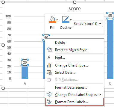
1. First, add data labels to your chart as needed. Then, right-click any of the data labels and select Format Data Labels from the context menu. See screenshot:

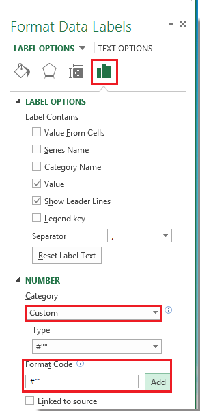
2. In the Format Data Labels dialog, click Number from the left pane. Next, choose Custom from the Category list box. Enter the custom format code #"" into the Format Code text box, and click Add to save it to the type list. See screenshot:

Note: In Excel 2013 or newer, after right-clicking on any data label and selecting Format Data Labels, expand Number in the formatting pane, select Custom, enter #"" as the Format Code, and click Add.
3. Click Close to exit the dialog. Now, any data label with a value of zero will be hidden from the chart display, leaving only nonzero values.
Tip: To restore zero data labels, return to the Format Data Labels dialog, select Number > Custom, and choose a standard number format such as #,##0;-#,##0 from the Type list.
This solution is particularly effective when you want a fast visual fix, and it works for most number-based charts (such as column, bar, line, etc.). However, if your data source is regularly updated with formulas or changing zero values, you may wish to explore formula-based or automated solutions below.
Caution: Custom number formatting will hide zeros visually in the chart, but the actual value remains zero in the background and in the source data.
Excel Formula - Hide zeros in chart with IF formula in source data
Another practical way to prevent zero data labels from appearing on your Excel chart is by modifying your source data using an IF formula. This method replaces zero values in the chart data range with blank cells, causing Excel's charting engine not to plot or label these points. This approach is especially useful when the chart references a dynamic data range or formulas, and you want to control which data is shown without additional formatting steps.
Applicable scenarios: Use this solution when you have control over the source data (or can create a helper column for the chart), and wish to completely exclude zero values from chart labels or the chart series itself.
Advantages: Simple, effective, ensures zeros are omitted from both the chart's data points and its labels.
Disadvantages: Requires you to either adjust existing data or add a helper column if you do not want to alter your original dataset.
To implement this solution:
1. In a new helper column or in your existing data range (e.g., suppose your original values are in column B starting from cell B2), enter the following formula in the corresponding cell of the helper column (e.g., cell C2):
=IF(A1=0,"",A1)This formula checks cell C2: if the value is zero, it returns a blank cell; otherwise, it returns the original value.
2. Press Enter to confirm the formula. Next, copy the formula down alongside your original data as needed by selecting the formula cell, dragging the fill handle, or using Ctrl+C/Ctrl+V.
3. Update your chart's data range to reference this new helper column (e.g., column C) so that the plotted series reflect the adjusted values.
- Right-click any existing data label in the chart and select "Format Data Labels".
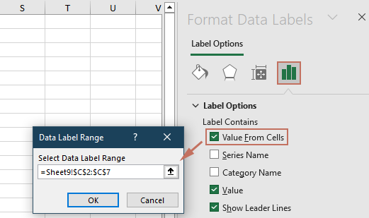
- Under Label Options, choose "Value From Cells". Then a dialog pops up, select the range of your helper column and click OK.
- Uncheck other label options such as "Value".


Now, Excel will not display data labels for zero values, because the cells in the chart data range are truly blank (not zero). As a reminder, ensure that blanks are not being interpreted as zeros in your chart settings (e.g., for line or scatter charts, check “Hidden and Empty Cell Settings” via Select Data → Hidden and Empty Cells).
Error reminder: If your formula column contains errors like #VALUE! in any cell, those points may also be omitted or display error labels on the chart—ensure your formula works for all rows.
VBA Code - Automatically hide zero data labels in chart
For larger datasets, frequently updated charts, or repeated reporting, using VBA provides a convenient and efficient way to automatically hide or remove zero data labels from an Excel chart. The VBA solution is suitable when you want to automate the process or handle multiple charts at once without manual formatting.
Applicable scenarios: This approach is best suited for users comfortable with running macros, or when managing complex and repetitive charting tasks across multiple Excel workbooks.
Advantages: Automates the hiding of zero data labels, saving time and reducing the opportunity for manual errors. Works even when chart data changes or when creating dashboards with frequent updates.
Disadvantages: Requires enabling macros, and an understanding of basic VBA procedures. Changes made by VBA may need to be refreshed if the data or chart series are updated after execution.
How to use this VBA solution:
1. On the Excel ribbon, click Developer > Visual Basic to open the VBA editor. In the VBA window, click Insert > Module, and paste the following code into the newly created module:
Sub HideZeroDataLabels()
'Updated by extendoffice 2025/7/11
    Dim cht As Chart
    Dim s As Series
    Dim pt As Point
    Dim xTitleId As String

    On Error Resume Next
    xTitleId = "KutoolsforExcel"

    Set cht = Application.ActiveChart
    If cht Is Nothing Then
        MsgBox "Please activate the chart from which you want to hide zero data labels.", vbExclamation, xTitleId
        Exit Sub
    End If

    For Each s In cht.SeriesCollection
        For Each pt In s.Points
            If pt.HasDataLabel Then
                If pt.DataLabel.Text = "0" Or pt.DataLabel.Text = "0%" Then
                    pt.DataLabel.Delete
                End If
            End If
        Next pt
    Next s
End Sub2. Return to your worksheet and activate the chart where you want to hide zero data labels (by clicking once on the chart border).
3. Return to the VBA editor and click the ![]() Run button (or press F5) to execute the macro. The macro will loop through all chart series and automatically hide any label with a value of zero, while leaving other data labels untouched.
Run button (or press F5) to execute the macro. The macro will loop through all chart series and automatically hide any label with a value of zero, while leaving other data labels untouched.
Practical tips: If your chart contains more than one data series, the macro will handle each series individually. You can also assign the macro to a custom button for easier repeated usage.
Error reminder: Ensure that you have enabled macros before running the code, and that the chart you want to process is currently activated, or the macro will prompt a warning.
Relative Articles:
Best Office Productivity Tools
Supercharge Your Excel Skills with Kutools for Excel, and Experience Efficiency Like Never Before. Kutools for Excel Offers Over 300 Advanced Features to Boost Productivity and Save Time. Click Here to Get The Feature You Need The Most...
Office Tab Brings Tabbed interface to Office, and Make Your Work Much Easier
- Enable tabbed editing and reading in Word, Excel, PowerPoint, Publisher, Access, Visio and Project.
- Open and create multiple documents in new tabs of the same window, rather than in new windows.
- Increases your productivity by 50%, and reduces hundreds of mouse clicks for you every day!
All Kutools add-ins. One installer
Kutools for Office suite bundles add-ins for Excel, Word, Outlook & PowerPoint plus Office Tab Pro, which is ideal for teams working across Office apps.
- All-in-one suite — Excel, Word, Outlook & PowerPoint add-ins + Office Tab Pro
- One installer, one license — set up in minutes (MSI-ready)
- Works better together — streamlined productivity across Office apps
- 30-day full-featured trial — no registration, no credit card
- Best value — save vs buying individual add-in