Check if value exists in another column in Excel – Full Guide
In Excel, verifying whether values from one column exist in another is a common task that can be approached through different methods, each suitable for either exact or partial matches. Highlighting these values can further assist in quickly identifying matches visually.
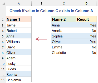
Suppose you have two columns of data, Column A and Column C, that both contain some duplicate values. Manually comparing these columns one by one is inefficient. This guide will explain how to check for value existence and highlight them in Excel.
Check if value exists in another column with formulas
To determine if a value in one column exists in another, the following formulas can do you a favor:
● Exact match:
To check for an exact match between values in two columns:
1. Please apply any one of the following formulas you like to a cell next to your data:
=IF(COUNTIF($A$2:$A$12, C2)>0, "Yes", "No")=IF(ISNUMBER(MATCH(C2, $A$2:$A$12, 0)), "Yes", "No")=IF(ISNA(VLOOKUP(C2, $A$2:$A$12, 1, FALSE)), "No", "Yes")=IF(ISNA(MATCH(C2, $A$2:$A$12, 0)), "No", "Yes")2. Then, drag the formula down to apply it to other cells. It checks each value in Column C against values in Column A. If there’s a match, it returns Yes, otherwise, No is displayed. See screenshot:

● Partial Match:
For partial matches, where you want to check if part of a text string in Column C exists within any string in Column A, please apply the following formulas:
1. Enter or copy any one of the following formulas into a cell to get the result:
=IF(SUMPRODUCT(--(ISNUMBER(SEARCH(C2, $A$2:$A$12)))), "Yes", "No")=IF(COUNTIF($A$2:$A$12,"*"&C2&"*")>0, "Yes", "No")
Highlight value if it is found in another column
Highlighting values in an Excel spreadsheet that appear in another column can significantly aid in data analysis, making it easier to spot duplicates or significant relationships between datasets. This section will explain how to highlight values found in another column using both Kutools' AI Aide and Excel's built-in Conditional Formatting, covering both exact and partial matches.
Highlight value if it is found in another column by using Kutools AI Aide
Kutools for Excel’s "AI Aide" feature can quickly determine whether a specific value exists in a designated column of your Excel sheet, handling both exact and partial matches with ease. Simply input your query, and Kutools AI Aide will analyze and execute the necessary actions. This powerful tool takes the hassle out of manually searching through columns and enables you to highlight matching values quickly, making it an indispensable aid for enhancing productivity and accuracy in your data management tasks.
After downloading and installing Kutools for Excel, click "Kutools AI" > "AI Aide" to open the "Kutools AI Aide" pane.
1. In the pane, type the following requirement into the chat box, and click "Send" button or press Enter key to send the question.
- Exact match:
- "Please check if value in Column C exists in Column A, highlight them with light blue color."
- Partial Match:
- "Please check if value in Column C exists in Column A (partial match), highlight them with light blue color."
2. After analyzing, click "Execute" button to run. Kutools AI Aide will process your request using AI and return the results directly in Excel.

Highlight value if it is found in another column with Conditional Formatting
Excel's Conditional Formatting feature is a powerful tool for visualizing relationships between data points by highlighting exact and partial matches. This section will walk you through the steps to set up Conditional Formatting for both exact and partial matches.
Step 1: Select Your Data
Select the range in your sheet where you want to apply the highlighting. This will typically be the column where you are looking for matches. Here, I will select the data in Column C.

Step 2: Apply Conditional Formatting
1. Click "Home" > "Conditional Formatting" > "New Rule", in the "New Formatting Rule" dialog box:
- Click "Use a formula to determine which cells to format" from the "Select a Rule Type" section;
- And then enter the following formula into the "Format values where this formula is true" text box;
=COUNTIF($A$2:$A$12, C2) > 0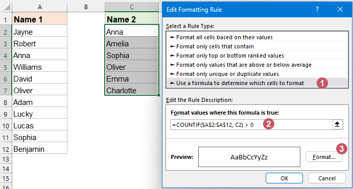
2. Then, click OK > OK to close the dialogs.
Result:
Now, you can see if a value in Column C exists in Column A, it will be highlighted.

To highlight values that partially match, adjust the formula as demonstrated below, and apply it into the Conditional Formatting.
=SUMPRODUCT(--(ISNUMBER(SEARCH(C2, $A$2:$A$12))))>0This will highlight if any part of the string in C2 is found within the range A2 to A12.

Whether you're aiming to verify exact or partial matches between columns in Excel, or highlight those matches, the methods outlined here—formulas, Kutools' AI Aide, and Conditional Formatting—offer robust solutions. You can choose the method that best suits your needs. If you're interested in exploring more Excel tips and tricks, our website offers thousands of tutorials, please click here to access them. Thank you for reading, and we look forward to providing you with more helpful information in the future!
Best Office Productivity Tools
Supercharge Your Excel Skills with Kutools for Excel, and Experience Efficiency Like Never Before. Kutools for Excel Offers Over 300 Advanced Features to Boost Productivity and Save Time. Click Here to Get The Feature You Need The Most...
Office Tab Brings Tabbed interface to Office, and Make Your Work Much Easier
- Enable tabbed editing and reading in Word, Excel, PowerPoint, Publisher, Access, Visio and Project.
- Open and create multiple documents in new tabs of the same window, rather than in new windows.
- Increases your productivity by 50%, and reduces hundreds of mouse clicks for you every day!
All Kutools add-ins. One installer
Kutools for Office suite bundles add-ins for Excel, Word, Outlook & PowerPoint plus Office Tab Pro, which is ideal for teams working across Office apps.
- All-in-one suite — Excel, Word, Outlook & PowerPoint add-ins + Office Tab Pro
- One installer, one license — set up in minutes (MSI-ready)
- Works better together — streamlined productivity across Office apps
- 30-day full-featured trial — no registration, no credit card
- Best value — save vs buying individual add-in