How to check if cell contains one of several values in Excel?

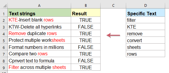
Supposing, you have a list of text strings in column A, now, you want to test each cell if it contains one of several values based on another range D2:D7. If it contains any of the specific text in D2:D7, it will display True, otherwise, it will show False as following screenshot shown. This article, I will talk about how to identify a cell if it contains one of several values in another range.

Check if a cell contains one of several values from a list with formulas

Display the matches if cell contains one of several values from a list with formulas

Highlight the matches if cell contains one of several values from a list with a handy feature

Check if a cell contains one of several values from a list with formulas

To check if a cell content contains any one of the text values in another range, the following formulas may help you, please do as this:

Enter the below formula into a blank cell where you want to locate the result, B2, for instance, then drag the fill handle down to the cells that you want to apply this formula, and if the cell has any of the text values in another specific range, it will get True, otherwise, it will get False. See screenshot:

Tips:

1. If you would like use “Yes” or “No’ to indicate the result, please apply the following formula, and you will get the following result as you need, see screenshot:

2. In the above formulas, D2:D7 is the specific data range which you want to check the cell based on, and A2 is the cell that you want to check.

Display the matches if cell contains one of several values from a list with formulas

Sotimes, you may want to check if a cell contains a value in the list and then returns that value, if multiple values match then all matching values in the list are displayed as below screenshot shown.How could you solve this task in Excel?

To display all matching vaues if the cell contains one of the specific text, please apply the below formula:

Note: In the above formula, D2:D7 is the specific data range which you want to check the cell based on, and A2 is the cell that you want to check.

Then, press Ctrl + Shift + Enter keys together to get the first result, and then drag the fill handle down to the cells that you want to apply this formula, see screenshot:

Tips:

The above TEXTJOIN function only available for Excel 2019 and Office 365, if you have earlier Excel versions, you should apply the below formula:

Note: In the above formula, D2:D7 is the specific data range which you want to check the cell based on, and A2 is the cell that you want to check.

Then, press Ctrl + Shift + Enter keys together to get the first result, and then drag the formula cell to right side until blank cell is displayed, and then go on dragging the fill handle down to other cells, and all matching values have been displayed as below screenshot shown:

Highlight the matches if cell contains one of several values from a list with a handy feature

If you want to highlight a specific font color for the matching values if cell contains one of several values from another list, this section, I will introduce an easy feature, Mark Keyword of Kutools for Excel, with this utility, you can highlight the specific one or more keywords at once within the cells.

After installing Kutools for Excel, please do as follows:

1. Click Kutools > Text > Mark Keyword, see screenshot:

2. In the Mark Keyword dialog box, please do the following operations:

• Select the data range that you want to highlight the matching texts from the Range textbox;
• Select the cells contains the keywords that you want to highlight based on, you can also enter the keywords manually (separate by comma) into the Keyword text box
• At last, you should specify a font color for highlighting the texts by check Mark keyword colors option. 

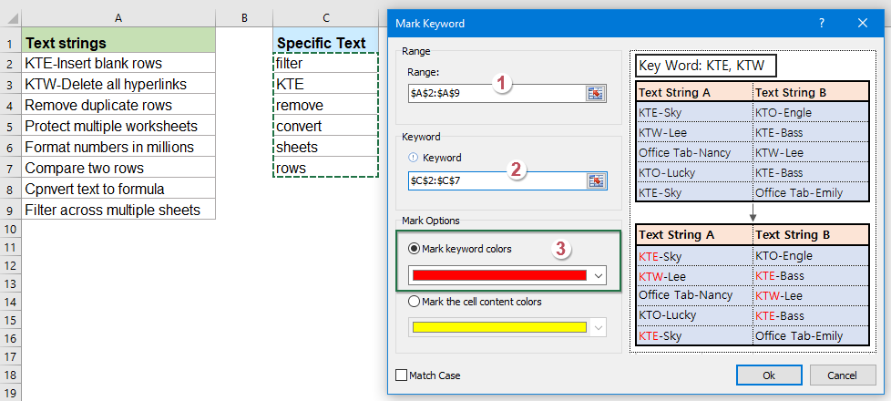
3. Then, click Ok button, all matching texts have been highlighted as below screenshot shown:

More relative articles:

---

The Best Office Productivity Tools

Kutools for Excel Solves Most of Your Problems, and Increases Your Productivity by 80%

• Reuse: Quickly insert complex formulas, charts and anything that you have used before; Encrypt Cells with password; Create Mailing List and send emails...
• Super Formula Bar (easily edit multiple lines of text and formula); Reading Layout (easily read and edit large numbers of cells); Paste to Filtered Range...
• Merge Cells/Rows/Columns without losing Data; Split Cells Content; Combine Duplicate Rows/Columns... Prevent Duplicate Cells; Compare Ranges...
• Select Duplicate or Unique Rows; Select Blank Rows (all cells are empty); Super Find and Fuzzy Find in Many Workbooks; Random Select...
• Exact Copy Multiple Cells without changing formula reference; Auto Create References to Multiple Sheets; Insert Bullets, Check Boxes and more...
• Extract Text, Add Text, Remove by Position, Remove Space; Create and Print Paging Subtotals; Convert Between Cells Content and Comments...
• Super Filter (save and apply filter schemes to other sheets); Advanced Sort by month/week/day, frequency and more; Special Filter by bold, italic...
• Combine Workbooks and WorkSheets; Merge Tables based on key columns; Split Data into Multiple Sheets; Batch Convert xls, xlsx and PDF...
• More than 300 powerful features. Supports Office / Excel 2007-2021 and 365. Supports all languages. Easy deploying in your enterprise or organization. Full features 30-day free trial. 60-day money back guarantee.

Read More... Free Download... Purchase... 

---

Office Tab Brings Tabbed interface to Office, and Make Your Work Much Easier

• Enable tabbed editing and reading in Word, Excel, PowerPoint, Publisher, Access, Visio and Project.
• Open and create multiple documents in new tabs of the same window, rather than in new windows.
• Increases your productivity by 50%, and reduces hundreds of mouse clicks for you every day!

Read More... Free Download... Purchase...