How to vlookup numbers stored as text in Excel?
When using VLOOKUP in Excel, encountering mismatched formats—specifically, when a lookup value is stored as text while the lookup column has numbers, or vice versa—can lead to lookup failures or errors. This formatting mismatch is a common issue, especially when data originates from external sources, is imported, or when working with large and collaborative datasets. Resolving these mismatches is essential to ensure VLOOKUP operates as expected and helps you retrieve the correct information. This step-by-step guide introduces several practical solutions to address these formatting inconsistencies, ensuring reliable and accurate lookups regardless of how numbers are stored in your workbook.
This article will demonstrate effective ways to handle such errors, including formula adjustments, built-in Excel tools, and VBA automation for bulk or automated processing. We also discuss the benefits and considerations of each method, helping you choose the most suitable approach for your scenario.
- Vlookup numbers stored as text with formulas
- Quickly fix format mismatches with Kutools for Excel
- VBA Macro: Standardize Formats Before VLOOKUP
- Other Built-in Excel Methods: Use 'Text to Columns' to Fix Data Formats
Vlookup numbers stored as text with formulas
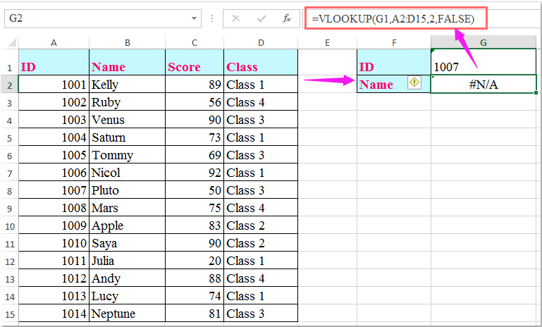
If your lookup data includes numbers stored as text in one place and actual numbers in another, VLOOKUP can fail to find matches due to this format inconsistency. One of the most direct solutions is to use Excel formulas that convert the lookup value or the lookup column to a consistent format on the fly. This approach works well in most worksheet operations, is easy to apply, and keeps your original data unchanged.
For example, if your lookup value is stored as text, while the corresponding field in the table is formatted as a number, you can use the VALUE function to convert the text to a number within the VLOOKUP formula.
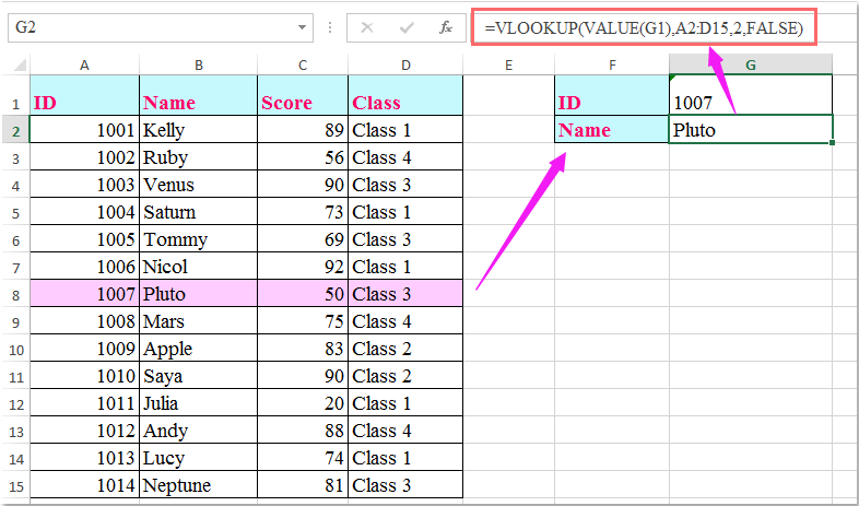
Enter the following formula in a blank cell where you want to display the result:
=VLOOKUP(VALUE(G1),A2:D15,2,FALSE)After entering the formula, press the Enter key to retrieve the value corresponding to your criteria, as illustrated in the screenshot below:
Parameter explanation and tips:
- G1: The cell containing the value you want to look up (can be either text or number).
- A2:D15: The range of your data table that includes the lookup column and the columns containing the information you want returned.
- 2: The column number (from the leftmost column of the table range) for the result you want to return.
Be mindful to check for leading/trailing spaces in lookup values, as these can also result in lookup failures. Consider combining the TRIM function if your data may contain extra spaces.
If the lookup value is a real number (number format), but the corresponding field in the table is stored as text, you need to convert the number to text before performing the lookup. The TEXT function is suitable for this scenario:
=VLOOKUP(TEXT(G1,0),A2:D15,2,FALSE)Enter this in your target cell, press Enter, and the correct result will be returned as shown below:
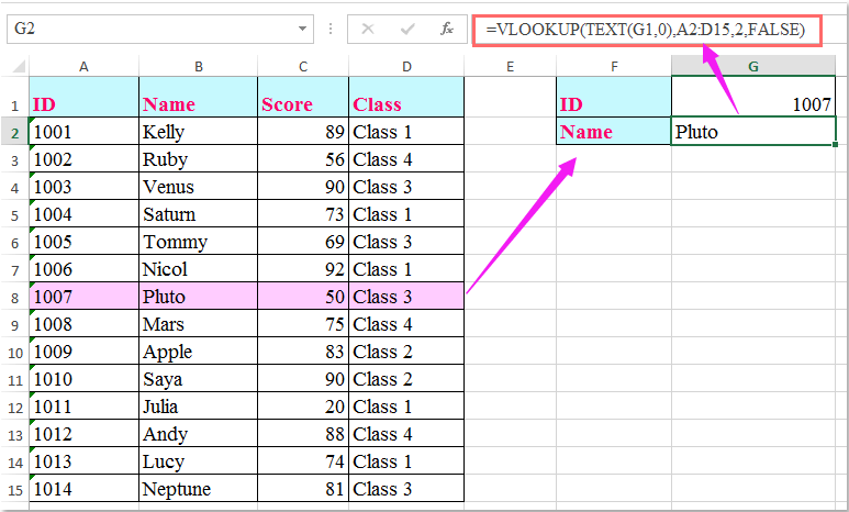
Here, the number format code “0” inside the TEXT function ensures your number is converted to a plain text value prior to matching.
If you are unsure about the possible formats of your lookup values or you expect both text and numbers to occur in your lookup column, you can nest both approaches using the IFERROR function to handle all possibilities seamlessly:
=IFERROR(VLOOKUP(VALUE(G1),A2:D15,2,0),VLOOKUP(TEXT(G1,0),A2:D15,2,0))Enter this formula in your result cell. It will first try the lookup by converting your value to a number; if that fails (for example, if the value cannot be coerced into a number), it will then try to convert your value to text and look it up again. This is especially useful in data sets with mixed formats or in shared files where data entry standards are not uniform.
After entering any of the above formulas, remember to copy the formula down to adjacent cells if you need to apply it to multiple lookup values—simply select the cell, drag the fill handle down, or use Ctrl+C and Ctrl+V as needed. For large tables, using these formulas helps ensure reliable matching without altering your original database.
This method provides a flexible and universally applicable solution for most worksheet-based lookups. However, for very large data sets or when you need to process many records automatically, you might consider using automation tools like VBA for even greater efficiency.
Quickly fix format mismatches with Kutools for Excel
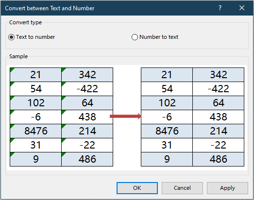
If you prefer a faster, no-formula solution, Kutools for Excel offers a user-friendly tool called Convert between Text and Number. This feature allows you to convert numbers stored as text into real numbers—or vice versa—with just a few clicks. It’s especially helpful when resolving format issues before performing lookups like VLOOKUP or MATCH.
After installing Kutools for Excel, please do as follow.
- Select the range that contains your problematic data (e.g., numbers stored as text).
- Go to "Kutools" > "Content" > "Convert between Text and Number".
- In the popup dialog:
- Choose "Text to number" if you're fixing lookup failures due to text-formatted numbers. (Or select "Number to text" if the lookup values are stored as text.)
- Click "OK" to immediately convert the data format.
- Choose "Text to number" if you're fixing lookup failures due to text-formatted numbers.

After converting text to numbers, the converted cells will behave as true numbers and no longer show green triangle indicators for inconsistency.
This approach eliminates the need for helper columns, formulas, or VBA—making it ideal for quick cleanup before applying VLOOKUP.
Kutools for Excel - Supercharge Excel with over 300 essential tools, making your work faster and easier, and take advantage of AI features for smarter data processing and productivity. Get It Now
VBA Macro: Standardize Formats Before VLOOKUP
For users who regularly work with large datasets, receive externally-sourced files, or require repeated automation, using a simple VBA macro can programmatically standardize the data format in both the lookup value column and the lookup table column. This way, you ensure all data is converted to either text or number before you run VLOOKUP, eliminating matching errors due to format mismatch. VBA is especially useful for bulk processing, saving manual adjustments, and ensuring data consistency through automation.
Advantages: Automation of formatting for large data ranges or frequent workflows; minimizes the risk of missing or inconsistent formatting; suitable for repetitive tasks.
Disadvantages: Not suitable for users with macro restrictions or those unfamiliar with VBA macro usage.
Here’s how you can use a macro to standardize cell formats:
1. Go to the Developer tab and click Visual Basic to open the VBA editor. In the new window, click Insert > Module, then copy and paste the following code into the module area:
Sub StandardizeLookupFormats()
    ' Ask the user to select the lookup column and choose a target format
    Dim rng As Range
    Dim userChoice As Integer
    Dim xTitleId As String

    On Error Resume Next
    xTitleId = "KutoolsforExcel"

    Set rng = Application.InputBox("Select the range to standardize (lookup or data column):", xTitleId, Type:=8)
    If rng Is Nothing Then Exit Sub

    userChoice = MsgBox("Convert selected data to Number? (Click Yes to convert to Number, No to convert to Text)", vbYesNoCancel, xTitleId)

    If userChoice = vbYes Then
        For Each cell In rng
            If IsNumeric(cell.Value) Then
                cell.Value = Val(cell.Value)
                cell.NumberFormat = "General"
            End If
        Next
    ElseIf userChoice = vbNo Then
        For Each cell In rng
            If Not IsEmpty(cell.Value) Then
                cell.Value = CStr(cell.Value)
                cell.NumberFormat = "@"
            End If
        Next
    Else
        Exit Sub
    End If
End Sub
2. Close the VBA editor. To run the macro, return to Excel, press Alt+F8, select StandardizeLookupFormats, and click Run.
Operation details and tips:
- This macro will prompt you to select the column (either your LOOKUP range or TABLE range) that you wish to standardize.
- After selection, it will ask if you want to convert the range to numbers (click Yes) or to text (click No). Select the same format for both your lookup and table columns to ensure VLOOKUP will match reliably.
- After running this macro, you may need to recalculate the worksheet (press F9) or re-apply your VLOOKUP formulas if results do not appear immediately.
- If you receive an error that macros are disabled, enable macros in your Excel settings before proceeding.
This solution is ideal for recurring data imports, or when cleaning up inconsistent columns in large datasets prior to applying VLOOKUP or other lookup operations.
Other Built-in Excel Methods: Use 'Text to Columns' to Fix Data Formats
A quick way to align number and text formats in Excel is to use the Text to Columns feature. This built-in tool is often used to split data but can also force a format conversion without editing formulas, making it helpful when you want a one-time fix or when dealing with straightforward lists.
Pros: Very easy, no formulas or code needed, preserves original data structure; Cons: Best for one-off corrections, doesn’t auto-update if data changes.
To use this method to convert numbers stored as text (or vice versa) in a column:
- Select the column with the suspected mismatched format (e.g., your lookup column or the column referenced by VLOOKUP).
- On the Data tab, click Text to Columns.
- In the wizard, choose Delimited, then click Next.
- Deselect all delimiter checkboxes (as you are not splitting the data); click Next.
- In Column Data Format, select General (to force Excel to recognize numbers as numbers) or select Text (to convert numbers to text).
- Click Finish to complete the process.
Once done, your data will have its format forcibly aligned to either number or text, resolving VLOOKUP mismatches. Always check a few cells to confirm that the conversion worked as expected. If necessary, repeat the process for both your lookup column and your lookup values to maximize consistency.
Practical reminders: “Text to Columns” modifies data directly, so it may overwrite cell contents if you have existing data to the immediate right. Consider copying your column to a blank area first if unsure, and always save a backup of your file before using bulk data tools.
Best Office Productivity Tools
Supercharge Your Excel Skills with Kutools for Excel, and Experience Efficiency Like Never Before. Kutools for Excel Offers Over 300 Advanced Features to Boost Productivity and Save Time. Click Here to Get The Feature You Need The Most...
Office Tab Brings Tabbed interface to Office, and Make Your Work Much Easier
- Enable tabbed editing and reading in Word, Excel, PowerPoint, Publisher, Access, Visio and Project.
- Open and create multiple documents in new tabs of the same window, rather than in new windows.
- Increases your productivity by 50%, and reduces hundreds of mouse clicks for you every day!
All Kutools add-ins. One installer
Kutools for Office suite bundles add-ins for Excel, Word, Outlook & PowerPoint plus Office Tab Pro, which is ideal for teams working across Office apps.
- All-in-one suite — Excel, Word, Outlook & PowerPoint add-ins + Office Tab Pro
- One installer, one license — set up in minutes (MSI-ready)
- Works better together — streamlined productivity across Office apps
- 30-day full-featured trial — no registration, no credit card
- Best value — save vs buying individual add-in