How to vlookup and return multiple values without duplicates in Excel?
When working with data in Excel, you may sometimes need to return multiple matching values for a specific lookup criterion. However, the default VLOOKUP function only retrieves a single value. In situations where multiple matches exist, and you want to display them in a single cell without duplicates, you can use alternative methods to achieve this.
Vlookup and return multiple matching values without duplicates in Excel
Return multiple matching values without duplicates with TEXTJOIN and FILTER functions
If you’re using Excel 365 or Excel 2021, you can leverage the TEXTJOIN and FILTER functions to achieve this easily. These functions allow dynamic filtering of data and concatenation of results into a single cell.
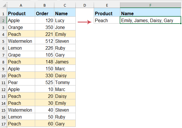
Please enter the below formula into a blank cell to output the result, and then press "Enter" key to get all matching values without duplicates. See screenshot:
=TEXTJOIN(", ", TRUE, UNIQUE(FILTER(C2:C17, A2:A17=E2)))
- FILTER(C2:C17, A2:A17=E2) extracts all names in Column C where the product in Column A matches the lookup value in E2.
- UNIQUE removes any duplicate values.
- TEXTJOIN(", ", TRUE, ...) combines the resulting unique values into a single cell, separated by commas.
Return multiple matching values without duplicates with a powerful feature
If you want to VLOOKUP and return multiple matching values without duplicates in Excel but find manual formulas or VBA too complex, "Kutools for Excel" offers an easy and efficient solution, with its "One-to-many Lookup" feature, you can quickly extract and combine all unique matching values into a single cell with just a few clicks.
Click "Kutools" > "Super Lookup" > "One-to-many Lookup (returns multiple results )" to open the "One-to-many Lookup" dialog box, then, specify the operations in the dialog box:
- Select the "Output range" and "Lookup values" in the textboxes separately;
- Select the table range that you want to use;
- Specify the key column and return column from the "Key Column" and "Return Column" drop down separately;
- Finally, click the "OK" button.


Result:
Now, you can see all matching values are extracted without duplicate item, see screenshot:
If you want to use a different delimiter to separate the data, you can click "Options" and select your desired delimiter. Additionally, you can perform other operations on the results, such as summing, averaging, and more.
Return multiple matching values without duplicates with User Defined Function
If you don't have Excel 365 or Excel 2021, you can use the User Defined Function provided below as an alternative. This method allows you to achieve similar results, such asreturning multiple matching values without duplicates, even in older versions of Excel.
- Hold down the "Alt" + "F11" keys to open the "Microsoft Visual Basic for Applications" window.
- Click "Insert" > "Module", and paste the following code in the "Module" Window.
VBA code: Vlookup and return multiple unique matched values:
Function VlookupUnique(lookupValue As String, lookupRange As Range, resultRange As Range, delim As String) As String Dim cell As Range Dim result As String Dim dict As Object Set dict = CreateObject("Scripting.Dictionary") For Each cell In lookupRange If cell.Value = lookupValue Then If Not dict.exists(resultRange.Cells(cell.Row - lookupRange.Row + 1, 1).Value) Then dict.Add resultRange.Cells(cell.Row - lookupRange.Row + 1, 1).Value, True result = result & delim & resultRange.Cells(cell.Row - lookupRange.Row + 1, 1).Value End If End If Next cell If Len(result) > 0 Then VlookupUnique = Mid(result, Len(delim) + 1) Else VlookupUnique = "" End If End Function - Save and close the code window, return to the worksheet, and enter the following formula, press "Enter" key to get the correct result as you need. See screenshot:
=VlookupUnique(E2, A2:A17, C2:C17, ", ")

In summary, there are several effective ways to VLOOKUP and return multiple matching values without duplicates in Excel, choose the method that best suits your needs and Excel version. With these techniques, you can easily return multiple matching values without duplicates in Excel. If you're interested in exploring more Excel tips and tricks, our website offers thousands of tutorials.
Best Office Productivity Tools
Supercharge Your Excel Skills with Kutools for Excel, and Experience Efficiency Like Never Before. Kutools for Excel Offers Over 300 Advanced Features to Boost Productivity and Save Time. Click Here to Get The Feature You Need The Most...
Office Tab Brings Tabbed interface to Office, and Make Your Work Much Easier
- Enable tabbed editing and reading in Word, Excel, PowerPoint, Publisher, Access, Visio and Project.
- Open and create multiple documents in new tabs of the same window, rather than in new windows.
- Increases your productivity by 50%, and reduces hundreds of mouse clicks for you every day!
All Kutools add-ins. One installer
Kutools for Office suite bundles add-ins for Excel, Word, Outlook & PowerPoint plus Office Tab Pro, which is ideal for teams working across Office apps.
- All-in-one suite — Excel, Word, Outlook & PowerPoint add-ins + Office Tab Pro
- One installer, one license — set up in minutes (MSI-ready)
- Works better together — streamlined productivity across Office apps
- 30-day full-featured trial — no registration, no credit card
- Best value — save vs buying individual add-in