How to sort dynamic data in Microsoft Excel?
When managing ever-changing data sets, such as inventory records for a stationary shop, sorting the information efficiently is essential for accurate reporting and quick analysis. However, manually re-sorting your data every time an update occurs can be both time-consuming and error-prone. The need arises: how can you keep your Excel lists sorted automatically, so whenever underlying data changes—such as quantity adjustments or new entries—your sorted results reflect the most current information without manual intervention?
This article details several practical methods to achieve automatic sorting of dynamic data in Excel. You'll learn both formula-based approaches and VBA automation, along with built-in modern Excel tools that help you keep your tables sorted as data evolves. These methods are suitable for scenarios such as stock management, sales tracking, grading, or any task where live, sorted data is critical.
➤ Sort dynamic data in Excel with formula
➤ Automatically sort data using Worksheet Change event (VBA)
➤ Use Excel Table (“Format as Table”) for easier sorting
➤ Sort with SORT or SORTBY dynamic array functions (Excel365/2019+)

Sort dynamic data in Excel with formula
This method works in all modern versions of Excel and applies best when you want to keep an automatically updated, sorted copy of your data alongside your original table. The approach relies on assigning ranks and then looking up values based on those ranks, so the sorted table stays up to date as your input changes.
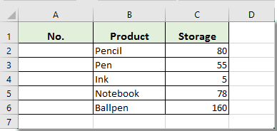
For example, suppose you are managing the inventory storage quantities for several types of stationery items. To have your table instantly reflect any changes in quantities and show products in descending order by storage, follow these steps:
1. Insert a new column at the beginning of the original data set. In the sample scenario, insert a column titled “No.” before the original data, as illustrated below:

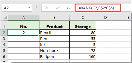
2. In cell A2 (the top cell under “No.”, assuming your data range is A2:C6), enter the following formula to calculate the ranking of each product based on its storage number. This allows Excel to assign a unique order to each item using the storage field:
=RANK(C2, C$2:C$6)Press Enter after typing the formula. The RANK function compares the storage value in C2 against the full range C2:C6, assigning a ranking number (with 1 being the highest storage). If you have more than five items, adjust C6 to cover the needed range.

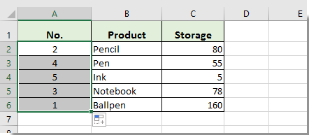
3. Keep cell A2 selected. Drag the Fill Handle down to cell A6 (or the last row of your data) to apply the ranking formula to all items in your list.

4. To create the dynamically sorted table, first copy the header row of your original data and paste it into a new location (for example, E1:G1). In the new “Desired No.” column (E2:E6 in this example), enter a sequential list of numbers matching the rankings (1, 2, 3, …). This sequence sets up the order for retrieval.

5. In cell F2 (beside “Product” in the new table), enter the following VLOOKUP formula to retrieve the product name corresponding to each rank number, then press Enter:
=VLOOKUP(E2, A$2:C$6, 2, FALSE)This formula searches for the given rank in column A and returns the associated product name from the second column.

6. Drag the Fill Handle from F2 down to F6 to fill in all product names. To fill in the sorted storage numbers, select F2:F6, then drag the Fill Handle right into G2:G6.
Your new table will display the products in descending order by storage value, always reflecting changes from your original table:

For example, if your stationery shop receives a delivery and you update the storage amount for “Pen” from 55 to 200 in your original list, the sorted table will instantly reposition the Pen entry to reflect its new rank and quantity—no manual sorting required. This solution automates list maintenance, reducing manual errors and keeping your key reports accurate.

Notes:
- Duplicate values (ties): If there are ties in the storage numbers, a simple
RANKwill assign the same rank to multiple rows andVLOOKUPwill only return the first match. For a stable order, replace Step 2 with this tie-breaker formula in A2 (then fill down):
=RANK(C2, C$2:C$6) + COUNTIF($C$2:C2, C2) - 1C$2:C$6, A$2:C$6) as your list grows. Converting the source to an Excel Table can simplify maintenance (structured references).Tips:
- On Microsoft 365 / Excel 2019+, consider using
SORT/SORTBYfor a more direct dynamic sort. - If you prefer to avoid helper columns, an advanced alternative is
INDEX/MATCH(orXLOOKUP) combined withSMALL/ROWto generate an ordered list, though it’s less readable and harder to maintain.
Tips & troubleshooting: Double-check your formula ranges to ensure all new or removed items are included as your original list changes size. You may need to adjust your references (e.g., C$2:C$10 instead of C$2:C$6) if you expand the list. For frequent list size changes, consider converting your data to an Excel Table and referencing table column names instead of cell ranges.
Automatically sort data using Worksheet Change event (VBA)
This solution is helpful when you want the original table to stay sorted in place—any user edits or new entries instantly trigger a reordering of the rows. It reduces manual sorting and works well for shared lists, inventory logs, and other frequently updated records.
Pros: Keeps the source data always sorted; no extra table or copying; applies to any number of columns.
Cons: Requires macros; anyone editing the file needs macro-enabled Excel.
Example scenario: A stationery store tracks stock in a table. Whenever someone changes a storage quantity, the corresponding row is automatically moved into proper rank order.
Use with caution: This method directly affects your data layout—keep backups or versioning if necessary.
To implement:
1. Right-click the sheet tab you want to auto-sort, and choose View Code.
2. In the worksheet’s code window (not a standard module), paste the following code:
Private Sub Worksheet_Change(ByVal Target As Range)
    On Error Resume Next
    Dim SortRange As Range
    ' Adjust your range as appropriate (example: A1:C6 includes headers)
    Set SortRange = Range("A1:C6")
    ' Sort by Storage in descending order (assuming Storage is in column C)
    SortRange.Sort Key1:=SortRange.Columns(3), Order1:=xlDescending, Header:=xlYes
End Sub
3. Close the VBA editor. Now, whenever data within A1:C6 is modified, Excel automatically re-sorts the entire range by the “Storage” column (column C) in descending order.
Notes:
- Update
Range("A1:C6")to match your real table (include headers). - This macro must live in the worksheet module (e.g., Sheet1 (Code)), not in a standard module.
- Save the workbook as
.xlsmand ensure macros are enabled, or the auto-sort will not run.
Tips:
- To sort by a different column, change the
Columns(3)argument to the desired index. - Need ascending order? Change
Order1:=xlDescendingtoxlAscending. - If your range grows, periodically expand the fixed address (e.g., to
A1:C1000) or convert the range to an Excel Table and update the macro to the table’s address.
Parameter explanation & troubleshooting: The macro sorts the fixed range you specify by the chosen column, assuming a header row. If sorting doesn’t occur, confirm macros are enabled and that you placed the code in the correct sheet module. If users edit outside the specified range, the sort won’t trigger—adjust the range to cover all editable rows.
Use Excel Table (“Format as Table”) for easier sorting
Converting your data range into an official Excel Table using the Format as Table feature provides several benefits for list management and sorting.
✅ Pros: Automatically updates structured references when adding or editing data, and provides sorting/filtering dropdowns for each column. You can sort the entire table instantly by clicking a column header dropdown. The table expands automatically when you add new rows.
⚠️ Cons: Sorting is not fully automatic — you still need to click to re-sort after changes, unless you add a VBA macro to trigger sorting automatically.
Typical scenario: In collaborative workbooks or large datasets where users need visual organization and quick row insertion, Excel Tables make routine sorting easier and less error-prone.
How to use:
- Select your data range and press Ctrl + T to convert it into an Excel Table. Make sure My table has headers is checked.
- Click the dropdown arrow in the header of the column you want to sort (e.g., Storage) and choose Sort Largest to Smallest or Sort Smallest to Largest.
If you want the sorting to happen automatically whenever the table is edited, attach a VBA macro (as described earlier) to the sheet containing the table. This combines the easy structure of Excel Tables with VBA automation.
💡 Tips: Excel Tables support structured references in formulas, making them easier to read and maintain as data grows. To clear a sort, use the column dropdown and select Clear Sort. If using VBA, ensure the macro references the correct table name (e.g., ListObjects("Table1")).
Sort with SORT or SORTBY dynamic array functions (Excel 365/2019+)
Modern versions of Excel (Excel 365, Excel 2019 and later) introduce dynamic array functions that can automatically generate a sorted version of your data in real time — no helper columns or VBA required.
✅ Pros: True real-time automatic sorting. Formulas “spill” results into adjacent cells as the original list grows or shrinks. Requires very few steps to set up.
⚠️ Cons: Only available in newer Excel versions. Output is a separate copy — your original range is not reordered.
Example scenario: You want a live-updating, sorted copy of your inventory list for dashboard display or reporting purposes, while preserving the input order for editing or data entry.
How to use:
Suppose your original data table is in range A2:C6 including headers in A1:C1. To generate a dynamically sorted table (by Storage, descending), enter this formula in any empty cell, such as E2:
=SORT(A2:C6, 3, -1)This produces a new, automatically sorted version of your original table, sorted by the third column (Storage) in descending order. Use -1 for descending and 1 for ascending.
For more refined sorting, such as secondary keys or custom criteria, use SORTBY:
=SORTBY(A2:C6, C2:C6, -1, B2:B6, 1)This sorts first by Storage (descending), then by Product (ascending).
After typing the formula, press Enter. Excel will “spill” the sorted data into adjacent rows and columns, automatically resizing as your source data changes.
💡 Tips:
- If adjacent cells are not empty, you’ll get a
#SPILL!error — ensure enough blank space for the output. - For data on another sheet, include the sheet name, e.g.,
=SORT(Sheet1!A2:C100, 3, -1). - If your source may grow, reference a larger range or define it as an Excel Table for structured referencing.
With these dynamic array methods, sorting and updating large lists for reporting or dashboards becomes effortless — the output is always up to date with no extra steps.

Unlock Excel Magic with Kutools AI
- Smart Execution: Perform cell operations, analyze data, and create charts—all driven by simple commands.
- Custom Formulas: Generate tailored formulas to streamline your workflows.
- VBA Coding: Write and implement VBA code effortlessly.
- Formula Interpretation: Understand complex formulas with ease.
- Text Translation: Break language barriers within your spreadsheets.
Best Office Productivity Tools
Supercharge Your Excel Skills with Kutools for Excel, and Experience Efficiency Like Never Before. Kutools for Excel Offers Over 300 Advanced Features to Boost Productivity and Save Time. Click Here to Get The Feature You Need The Most...
Office Tab Brings Tabbed interface to Office, and Make Your Work Much Easier
- Enable tabbed editing and reading in Word, Excel, PowerPoint, Publisher, Access, Visio and Project.
- Open and create multiple documents in new tabs of the same window, rather than in new windows.
- Increases your productivity by 50%, and reduces hundreds of mouse clicks for you every day!
All Kutools add-ins. One installer
Kutools for Office suite bundles add-ins for Excel, Word, Outlook & PowerPoint plus Office Tab Pro, which is ideal for teams working across Office apps.
- All-in-one suite — Excel, Word, Outlook & PowerPoint add-ins + Office Tab Pro
- One installer, one license — set up in minutes (MSI-ready)
- Works better together — streamlined productivity across Office apps
- 30-day full-featured trial — no registration, no credit card
- Best value — save vs buying individual add-in