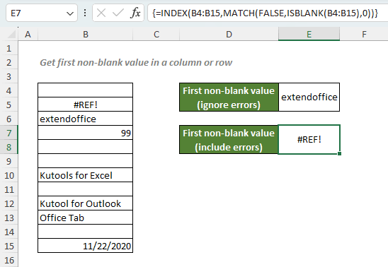
Get first non-blank value in a column or row
To retrieve the first value (the first cell that is not blank, ignoring errors) from a one-column or one-row range, you can use a formula based on INDEX and MATCH functions. However, if you don’t want to ignore the errors from your range, you can add the ISBLANK function to the above formula.

Get first non-blank value in a column or row ignoring errors
Get first non-blank value in a column or row including errors
Get first non-blank value in a column or row ignoring errors
To retrieve the first non-blank value in the list as shown above ignoring errors, you can use the INDEX function inside the MATCH function "INDEX((range<>0),0)" to find the cells that are not blank. And then use the MATCH function to locate the position of the first non-blank cell. The location will then be fed to the outer INDEX to retrieve the value at that position.
Generic syntax
=INDEX(range,MATCH(TRUE,INDEX((range<>0),0),0))
- range: The one-column or one-row range where to return the first non-blank cell with text or number values while ignoring errors.
To retrieve the first non-blank value in the list ignoring errors, please copy or enter the formula below in the cell E4, and press Enter to get the result:
=INDEX(B4:B15,MATCH(TRUE,INDEX((B4:B15<>0),0),0))

Explanation of the formula
=INDEX(B4:B15,MATCH(TRUE,INDEX((B4:B15<>0),0),0))
- INDEX((B4:B15<>0),0):The snippet evaluates each value in the range B4:B15. If a cell is blank, it will return a FALSE; If a cell contains an error, the snippet will return the error itself; And if a cell contains a number or text, a TRUE will be returned. Since the row_num argument of this INDEX formula is 0, so the snippet will return the array of values for the entire column like this: {FALSE;#REF!;TRUE;TRUE;FALSE;FALSE;TRUE;FALSE;TRUE;TRUE;FALSE;TRUE}.
- MATCH(TRUE,INDEX((B4:B15<>0),0),0) = MATCH(TRUE,{FALSE;#REF!;TRUE;TRUE;FALSE;FALSE;TRUE;FALSE;TRUE;TRUE;FALSE;TRUE},0): The match_type 0 forces the MATCH function to return the position of the first exact TRUE in the array. So, the function will return 3.
- INDEX(B4:B15,MATCH(TRUE,INDEX((B4:B15<>0),0),0)) = INDEX(B4:B15,3): The INDEX function then returns the 3rd value in the range B4:B15, which is extendoffice.
Get first non-blank value in a column or row including errors
To retrieve the first non-blank value in the list including errors, you can simply use the ISBLANK function to check the cells in the list if they are blank or not. Then INDEX will return the first non-blank value according to the position that MATCH provided.
Generic syntax
=INDEX(range,MATCH(FALSE,ISBLANK(range),0))
√ Note: This is an array formula that requires you to enter with Ctrl + Shift + Enter, except in Excel 365 and Excel 2021.
- range: The one-column or one-row range where to return the first non-blank cell with text, number or error values.
To retrieve the first non-blank value in the list including errors, please copy or enter the formula below in the cell E7, and press Ctrl + Shift + Enter to get the result:
=INDEX(B4:B15,MATCH(FALSE,ISBLANK(B4:B15),0))
Explanation of the formula
=INDEX(B4:B15,MATCH(FALSE,ISBLANK(B4:B15),0))
- ISBLANK(B4:B15): The ISBLANK function checks if the cells in the range B4:B15 are blank or not. If yes, a TRUE will be returned; If not, a FALSE will be returned. So, the function will generate an array like this: {TRUE;FALSE;FALSE;FALSE;TRUE;TRUE;FALSE;TRUE;FALSE;FALSE;TRUE;FALSE}.
- MATCH(FALSE,ISBLANK(B4:B15),0) = MATCH(FALSE,{TRUE;FALSE;FALSE;FALSE;TRUE;TRUE;FALSE;TRUE;FALSE;FALSE;TRUE;FALSE},0):The match_type 0 forces the MATCH function to return the position of the first exact FALSE in the array. So, the function will return 2.
- INDEX(B4:B15,MATCH(FALSE,ISBLANK(B4:B15),0)) = INDEX(B4:B15,2): The INDEX function then returns the 2nd value in the range B4:B15, which is #REF!.
Related functions
The Excel INDEX function returns the displayed value based on a given position from a range or an array.
The Excel MATCH function searches for a specific value in a range of cells, and returns the relative position of the value.
Related Formulas
Exact match with INDEX and MATCH
If you need to find out the information listed in Excel about a specific product, movie or a person, etc., you should make a good use of the combination of INDEX and MATCH functions.
Get first text value in a column
To retrieve the first text value from a one-column range, you can use a formula based on INDEX and MATCH functions as well as a formula based on the VLOOKUP function.
Locate first partial match with wildcards
There are cases that you need to get the position of the first partial match that contains specific number in a range of numeric values in Excel. In this case, a MATCH and TEXT formula that incorporates asterisk (*), the wildcard that matches any number of characters, will do you a favor. And if you also need to know the exact value at that position, you can add the INDEX function to the formula.
Lookup the first partial match number
There are cases that you need to get the position of the first partial match that contains specific number in a range of numeric values in Excel. In this case, a MATCH and TEXT formula that incorporates asterisk (*), the wildcard that matches any number of characters, will do you a favor. And if you also need to know the exact value at that position, you can add the INDEX function to the formula.
The Best Office Productivity Tools
Kutools for Excel - Helps You To Stand Out From Crowd
Kutools for Excel Boasts Over 300 Features, Ensuring That What You Need is Just A Click Away...
Office Tab - Enable Tabbed Reading and Editing in Microsoft Office (include Excel)
- One second to switch between dozens of open documents!
- Reduce hundreds of mouse clicks for you every day, say goodbye to mouse hand.
- Increases your productivity by 50% when viewing and editing multiple documents.
- Brings Efficient Tabs to Office (include Excel), Just Like Chrome, Edge and Firefox.