Excel MATCH Function
The Microsoft Excel MATCH function searches for a specific value in a range of cells, and returns the relative position of this value.
Syntax
=MATCH (lookup_value, lookup_array, [match_type])
Arguments
Lookup_value (Required): The specific value you want to match in the look_up array;
This argument can be a number, text, logical value or a cell reference to a value (number, text, or logical value)
Lookup_array (Required): A range of cells that contains the value you are searching for.
Match_type (optional): The type of match that the function will perform. It contains 3 types:
- 0 - Finds the first value exactly match to the lookup_value
- 1 - or omitted If the exact match value can’t be found, Match will find the largest value that is less than or equal to the look_up value.
The values in the look_up array argument must be in ascending order. - -1 - Finds the smallest value that is greater than or equal to the look_up value.
The values in the look_up array argument must be in descending order.
Return value
The MATCH function will return a number representing the position of a value you are searching for.Function notes
1. The MATCH function is not case-sensitive.
2. The Match function will return the #N/A error value when failing to find a match.
3. The MATCH function allows to use the wildcard characters in the lookup_value argument for approximate match.
Examples
Example 1: MATCH function for exact match
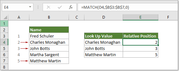
Please do as follows to return the positon of Charles Monaghan in range B3:B7.
Select a blank cell and enter the below formula into it and press the Enter key to get the result.
=MATCH(D4,B3:B7,0)
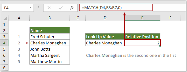
Note: In the formula, D4 contains the look up value; B3:B7 is the range of cells that contains the value you are searching for; number 0 means that you are looking for the exact match value.
Example 2: MATCH function for approximate match
This section is talking about using the MATCH function to do the approximate match searching in Excel.
As the below screenshot shown, you want to look for the position of number 2500 in range B3:B7, but there is no 2500 in the list, here I will show you how to return the position of the largest value that is less than 2500 in the list.
Select a blank cell, enter the below formula into it and then press the Enter key to get the result.
=MATCH(D4,B3:B7,1)
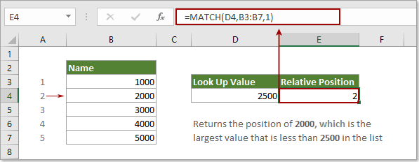
Then it will return the position of number 2000, which is the largest value that is less than 2500 in the list.
Note: In this case, all values in the list B3:B7 must be sorted in ascending order, otherwise, it will return #N/A error.
For returning the position of the smallest value (says 3000) that is greater than 2500 in the list, please apply this formula:
=MATCH(D4,B3:B7,-1)
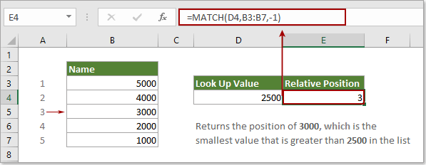
Note: All values in the list B3:B7 must be sorted in descending order in case of returning #N/A error.
Example 3: MATCH function for wildcard match in MATCH function
Besides, the MATCH function can perform a match using wildcards when the match type is set to zero.
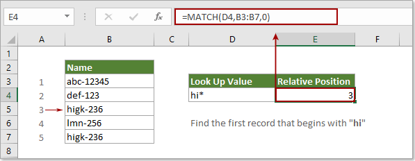
As the below screenshot shown, for getting the position of the value which begins with “hi”, please do as follows.
Select a blank cell, enter the below formula (you can replace the D4 directly with "hi*") into it and press the Enter key. It will return the position of the first match value.
=MATCH(D4,B3:B7,0)
Tip: The MATCH function is not case-sensitive.
More Examples
How to find next largest value in Excel?
How to find the longest or shortest text string in a column?
How to find highest value in a row and return column header in Excel?
The Best Office Productivity Tools
Kutools for Excel - Helps You To Stand Out From Crowd
Kutools for Excel Boasts Over 300 Features, Ensuring That What You Need is Just A Click Away...
Office Tab - Enable Tabbed Reading and Editing in Microsoft Office (include Excel)
- One second to switch between dozens of open documents!
- Reduce hundreds of mouse clicks for you every day, say goodbye to mouse hand.
- Increases your productivity by 50% when viewing and editing multiple documents.
- Brings Efficient Tabs to Office (include Excel), Just Like Chrome, Edge and Firefox.