Excel OFFSET Function
The Excel OFFSET function returns a reference to a cell or a range of cells that is offset from a specific cell by a given number of rows and columns.
Syntax
=OFFSET (reference, rows, cols, [height], [width])
Arguments
Reference (required): A cell or a range of adjacent cells you will set as the starting point.
Rows (required): The number of rows to move up (negative number) or down (positive number) from the starting point.
Cols (required): The number of columns to move left (negative number) or right (positive number) from the starting point.
Height (optional): The number of rows you want to return. The height must be a positive number.
Width (optional): The number of columns you want to return. The width must be a positive number.
Return value
The OFFSET function will return a cell reference offset from a given starting point.
Function notes
1. #VALUE! error value will return when the reference refer to a range of discontinuous cells.
2. #REF! error value will return when the rows and columns offset reference over the edge of the worksheet.
Examples
Example 1: Basic usage for the OFFSET function
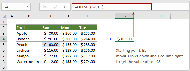
Return a reference to a cell with the below formula:
=OFFSET(B2,3,1)
In this case, B2 is the starting point, number 3 and 1 mean that to move 3 rows down and 1 column right from cell B2, and return the value in C5 finally. See screenshot:
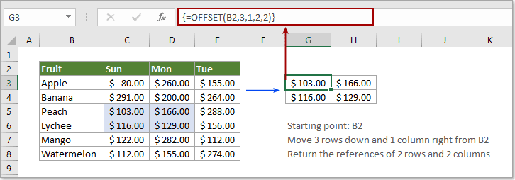
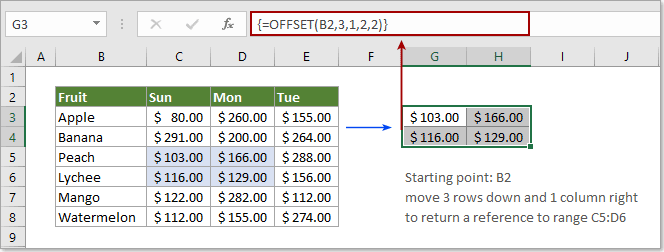
Return a reference to a range of cells with the below formula:
=OFFSET(B2,3,1,2,2)
In this case, you will get the results of 2 x 2 range that is 3 rows below and 1 column right of cell B2.
Note: #VALUE! Error will occur when you only selecting one cell to apply the OFFSET function for returning a range of cells. You need to select a 2 x 2 range (says 4 blank cells), enter the formula and press the Ctrl + Shift + Enter keys to get the results.
Example 2: Use the OFFSET function to sum a range of values
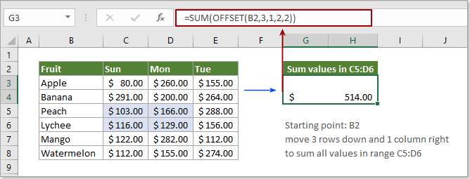
As we mentioned above, if you try to use the OFFSET function such as =OFFSET(B2,3,1,2,2) on its own in a single cell, it will return a #VALUE! Error. However, if you combine the SUM and OFFSET function as below screenshot shown, it will return the sum of values in range C5:D6 directly.
1. Select a blank cell, copy the below formula into it and press the Enter key to get the result.
=SUM(OFFSET(B2,3,1,2,2)))
Example 3: Sum columns based on certain criteria
As below screenshot shown, how to get the total sales of Mango from Sun to Tue? Please try as below.
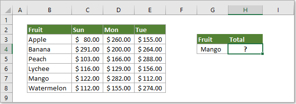
1. Select a blank cell, copy the below formula into it and press the Enter key to get the result.
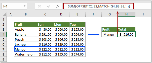
=SUM(OFFSET(C2:E2,MATCH(G4,B3:B8,),))
Notes:
1. In the above formula, MATCH(G4,B3:B8) is looking for Mango and returning its position in range B3:B8. Let’s see, Mango locates 5 rows below cell B2, so it returns the number 5;
2. As the MATCH result is 5, and the last comma here represents 0, the OFFSET function now is displaying as OFFSET(C2:E2,5,0), which means that the offset starts from range C2:E2, move 5 rows down and 0 column right to get the reference to range C7:E7;
3. Then the SUM function displays as SUM(C7:E7), and finally return the sum of values in range C7:E7.
More Examples
How to sum every n rows down in Excel?
The Best Office Productivity Tools
Kutools for Excel - Helps You To Stand Out From Crowd
Kutools for Excel Boasts Over 300 Features, Ensuring That What You Need is Just A Click Away...
Office Tab - Enable Tabbed Reading and Editing in Microsoft Office (include Excel)
- One second to switch between dozens of open documents!
- Reduce hundreds of mouse clicks for you every day, say goodbye to mouse hand.
- Increases your productivity by 50% when viewing and editing multiple documents.
- Brings Efficient Tabs to Office (include Excel), Just Like Chrome, Edge and Firefox.