How to find the max or min value based on criteria in Excel?
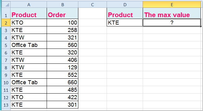
Suppose you have a data range with product names in column A and order quantities in column B. Now, you want to quickly identify the maximum or minimum order quantity for a specific product, such as "KTE", as shown in the screenshot below. Excel offers several approaches for extracting the max or min value based on one or several criteria.
Find the Max or Min value based on only one criterion
Find the Max or Min value based on multiple criteria
Excel MAXIFS and MINIFS functions (Excel 2019+)
Find the Max or Min value based on criterion with Pivot Table
Find the Max or Min value based on only one criterion
To return the max or min value with one criterion, you can use the MAX or MIN function together with an array formula.
This method is most useful if you need to quickly look up the highest or lowest value for a single, clearly defined condition—such as finding the best-selling product or the minimum sales amount of a single item.
1. Enter the following formula in the cell where you want the result (for example, in E2):
=MAX((A2:A13=D2)*B2:B13)
Tips: In this formula: A2:A13 specifies the range of cells that contains your criteria, D2 is the criteria you want to use (e.g., the product name "KTE"), and B2:B13 is the value range from which the result will be returned.
Be sure to use absolute or relative cell references appropriately if you plan to copy the formula elsewhere.
2. After entering the formula, press Ctrl + Shift + Enter (not just Enter). Excel will wrap your formula in curly braces { }, indicating that it is an array formula, and display the max value that matches your criterion. See screenshot:

Note: To obtain the minimum value based on a specific criterion, type this formula:
=MIN(IF(A2:A13=D2,B2:B13))Remember to confirm with Ctrl + Shift + Enter as well. The result will display the smallest quantity for the specified product.

If you receive a #VALUE! or similar error, check that your ranges are of equal size, your criteria cell contains the correct value, and that you have confirmed the formula with Ctrl + Shift + Enter instead of just Enter.

Unlock Excel Magic with Kutools AI
- Smart Execution: Perform cell operations, analyze data, and create charts—all driven by simple commands.
- Custom Formulas: Generate tailored formulas to streamline your workflows.
- VBA Coding: Write and implement VBA code effortlessly.
- Formula Interpretation: Understand complex formulas with ease.
- Text Translation: Break language barriers within your spreadsheets.
Find the Max or Min value based on multiple criteria
In cases where you need to find the max or min value that meets several conditions—such as a specific product in a particular month or region—you can use an array formula that includes multiple criteria within nested IF statements.
For example, consider the following data. Here, you want to find the maximum (or minimum) order quantity for product KTE in January.

1. Enter this formula into the cell where you want the result (such as H2):
=MAX(IF(A2:A13=F1,IF(B2:B13=F2,C2:C13)))
Tips: In this formula: A2:A13 contains your first criteria, B2:B13 provides the second criteria, F1 and F2 are the values for the criteria to match, and C2:C13 is the range to return the maximum value from. Adjust the ranges and criteria as needed for your dataset.
Use this structure when you have two or more filtering conditions. Make sure all ranges are the same length to avoid errors.
2. Press Ctrl + Shift + Enter after typing the formula, and the result will display the maximum value found for product and month matching your criteria. This process is especially useful when filtering data by combinations of fields such as category, region, or time period.

Note: For the minimum value under the same conditions, apply this formula:
=MIN(IF(A2:A13=F1,IF(B2:B13=F2,C2:C13)))Ensure you use Ctrl + Shift + Enter. If the formula doesn't output as expected, double-check the values in your criteria cells and make sure you didn’t include entire columns if there’s a blank or text in your value range.
Array formulas require careful attention to cell references and selection of the correct cell ranges. If results do not appear as expected, confirm that ranges have the same number of rows and your criteria cells contain the intended values.
Use MAXIFS and MINIFS Functions (Excel 2019+)
If you are using Excel 2019 or a later version, you can use the built-in MAXIFS and MINIFS functions to retrieve max or min values based on one or more conditions—without the need for array formulas or pressing Ctrl + Shift + Enter. This approach is more straightforward, especially when working with multiple criteria or if you want to avoid array syntax.
Applicable Scenarios: Use this method if you have access to Excel 2019 or newer, to simplify your formulas and reduce errors.
1. To get the maximum value for "KTE", enter this formula in your target cell (for example, E2):
=MAXIFS(B2:B13,A2:A13,D2)This formula finds the largest value in B2:B13 (order quantity) where the product in A2:A13 matches the value in D2 (e.g., "KTE").
2. Press Enter to confirm the formula. You do not need to use Ctrl + Shift + Enter. To apply this formula on other rows or for other products, simply adjust your criteria cell or copy down as needed.
To find the minimum value with one criterion, use:
=MINIFS(B2:B13,A2:A13,D2)Similarly, for multiple criteria, you can expand the formula. For example, to find the max order for product KTE in January (where the month values are in B2:B13 and the quantities are in C2:C13):
=MAXIFS(C2:C13,A2:A13,F1,B2:B13,F2)In this example, F1 is your product criterion and F2 is your month criterion. Adjust the fields based on your dataset.
Pivot Table Solution
Pivot tables offer an interactive way to quickly analyze large amounts of data and can instantly display the max or min values based on selected criteria. This solution is ideal if you need to summarize data by different categories (such as product, region, or date) and want to get a dynamic overview of highest or lowest values.
Applicable Scenarios: Use this method when you need flexible, interactive reports, or when collaborating and sharing insights with others who may prefer summary tables over formulas.
To set up a pivot table to extract the max or min by criteria:
1. Select your data range, including headers (for example, A1:B13).
2. Go to the Insert tab in the ribbon and click PivotTable.
3. In the dialog, choose where to place your pivot table (new worksheet is recommended) and click OK.
4. In the PivotTable Fields pane, drag the criteria field (such as Product) to the Rows area, and the value field (such as Order Quantity) to the Values area.
5. By default, the value will be summarized by Sum. Click on the drop-down arrow next to the field in the Values area, choose Value Field Settings, and then select Max or Min as needed. Click OK to confirm.
Now, the pivot table will display the maximum or minimum value for each criteria (for example, the highest or lowest order quantity for each product). You can further filter and group your data as needed by adding more fields to the Rows, Columns, or Filters areas.
Note: If your dataset updates, right-click the pivot table and select Refresh to ensure your calculations stay current.
Advantages: Pivot tables make it very intuitive to adjust criteria, drill down into details, and generate dynamic summaries without changing your underlying data or formulas. They are also particularly suited for large or complex datasets.
Related articles:
How to select max data/value with max function in Excel?
How to select the highest value and lowest value in Excel?
Best Office Productivity Tools
Supercharge Your Excel Skills with Kutools for Excel, and Experience Efficiency Like Never Before. Kutools for Excel Offers Over 300 Advanced Features to Boost Productivity and Save Time. Click Here to Get The Feature You Need The Most...
Office Tab Brings Tabbed interface to Office, and Make Your Work Much Easier
- Enable tabbed editing and reading in Word, Excel, PowerPoint, Publisher, Access, Visio and Project.
- Open and create multiple documents in new tabs of the same window, rather than in new windows.
- Increases your productivity by 50%, and reduces hundreds of mouse clicks for you every day!
All Kutools add-ins. One installer
Kutools for Office suite bundles add-ins for Excel, Word, Outlook & PowerPoint plus Office Tab Pro, which is ideal for teams working across Office apps.
- All-in-one suite — Excel, Word, Outlook & PowerPoint add-ins + Office Tab Pro
- One installer, one license — set up in minutes (MSI-ready)
- Works better together — streamlined productivity across Office apps
- 30-day full-featured trial — no registration, no credit card
- Best value — save vs buying individual add-in