How to Hide Duplicate Values and Rows in Excel
Duplicate data is common in Excel worksheets, especially when working with customer lists, inventory records, sales reports, or imported data. In many cases, you may want to temporarily conceal repeated values or display only unique records without permanently removing any information.
Depending on your goal, you might need to visually hide duplicate values, display only unique rows, focus on unique records within a specific subset of data, or review unique records from filtered results. In this tutorial, we'll explore several practical methods to accomplish these tasks while keeping your original dataset intact.
Visually hide duplicate records in a range
This section is for cases where you do not want to hide rows or remove data. You only want duplicate cells to disappear visually, while the original values remain in the worksheet. This is useful when you need to keep the full dataset for formulas, sorting, filtering, or review, but want duplicate values to be less visible.
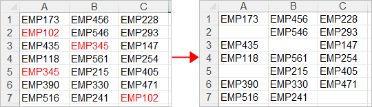
Hide duplicates with Conditional Formatting
This method applies formatting to all duplicate values, including the first occurrences, so they blend into the worksheet background.
- Select the range containing your data.
- Click Home > Conditional Formatting > Highlight Cells Rules > Duplicate Values.
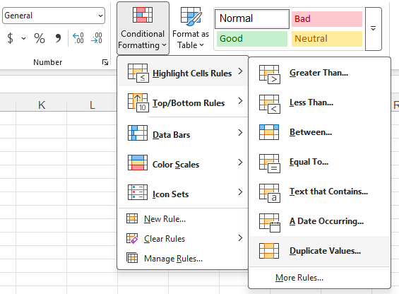
- In the Duplicate Values dialog box, choose Custom Format.
- On the Font tab, choose a font color that matches your worksheet background, such as white.
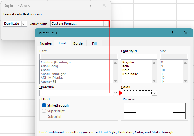
- Click OK twice.
Duplicate values will now become invisible while remaining in the worksheet.
Notes:
- This method only hides duplicates visually.
- The data still exists and can be used in formulas, sorting, and filtering.
- The built-in Duplicate Values rule treats all duplicate occurrences equally and cannot distinguish between the first occurrence and subsequent occurrences.
Pros
- Fast and easy to apply
- No formulas required
- Works on any selected range
Cons
- Cannot hide duplicates except the first occurrence
- Formatting may become confusing in shared workbooks
Hide duplicates with Kutools' Select Duplicate & Unique Cells
Kutools for Excel provides more control over duplicate identification. Unlike Excel's built-in duplicate formatting, it allows you to choose whether the first occurrence should be included.
- Select the data range.
- Click Kutools > Select > Select Duplicate & Unique Cells.
- In the dialog box, choose Single cell.
- In the rule section, choose one of the following options:
- Duplicates (Except 1st one)
- All duplicate (Including 1st one)
- Check the Fill font color option, and specify the font color as white.
- Click OK.
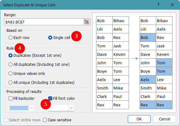
After clicking OK, all duplicates are formatted with the color you specified and visually hidden. Also, the duplicate cells are selected automatically, allowing you to perform further actions, such as deleting them, applying another format, copying them, or reviewing them directly.
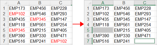
Pros
- Can distinguish between first and subsequent duplicates
- Easy to use
- No helper columns required
Cons
- Requires Kutools for Excel
Kutools for Excel - Packed with over 300 essential tools for Excel. Make Excel tasks faster, easier, and more efficient. Download now!
Hide duplicate rows
Sometimes you need to hide entire rows instead of individual duplicate values. This is common when each row represents a complete record, such as an order, customer, product, or transaction. In this case, hiding only the duplicate cells is not enough because the whole record should be removed from view.
Hide duplicate rows with Advanced Filter
Advanced Filter can display unique records while hiding duplicate records from view. When duplicate rows exist, Excel keeps the first occurrence visible and hides the remaining duplicate occurrences.
- Select your dataset. The selection must include the header row.
- Click Data > Advanced.
- In the Advanced Filter dialog box, choose Filter the list, in-place.
- Check Unique records only.
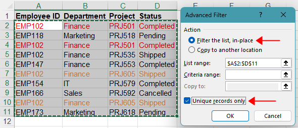
- Click OK.
Excel displays unique records and first occurrences only. Duplicate occurrences are hidden automatically.
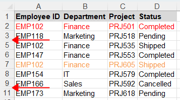
Pros
- Built into Excel
- No formulas required
- Quickly displays unique records
Cons
- Keeps first occurrences visible
- Must be reapplied when data changes
Hide duplicate rows with Kutools' Find Duplicates
Kutools for Excel provides a dedicated Find Duplicates feature for finding and hiding duplicate rows. It is useful when you want to compare full rows, or when you only want to compare selected columns, without preparing formulas or criteria ranges.
- Select your data range.
- Click Kutools > Find > Find Duplicates.
- Leave all checkboxes selected to find duplicate rows with completely identical values across all columns.Tip: If you want to hide rows when a specific column has duplicates, select only that column and leave other columns unchecked.
- Select Hide Duplicates.
- Click OK.
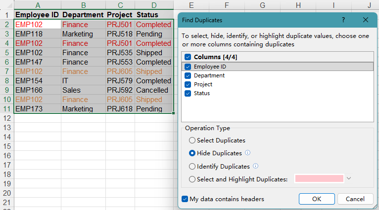
The duplicate rows, excluding the first occurrences, are hidden at once.
Pros
- Easy to use
- No formulas or helper columns required
- Supports selected columns
Cons
- Requires Kutools for Excel
- Keeps first occurrences visible
Kutools for Excel - Packed with over 300 essential tools for Excel. Make Excel tasks faster, easier, and more efficient. Download now!
Hide duplicate rows including first occurrences with COUNTIF and Filter
The two methods above keep the first occurrence visible. If you want to hide all rows that belong to duplicate groups, including the first occurrence, use a helper column and a formula.
- Insert a helper column beside your data.
- Enter one of the following formulas:
- To hide rows when values in Column A occur more than once, including the first occurrences:
=COUNTIF($A:$A,A2)>1 - To hide duplicate rows when all values in columns A to C are the same, including the first occurrences:
=COUNTIFS($A:$A,A2,$B:$B,B2,$C:$C,C2)>1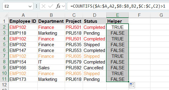
📝 Note:
The formula returns TRUE for rows that belong to a duplicate group (values that appear more than once in the dataset), and FALSE for rows that contain unique values only.
- To hide rows when values in Column A occur more than once, including the first occurrences:
- Click Data > Filter.
- Filter the helper column for FALSE.
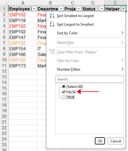
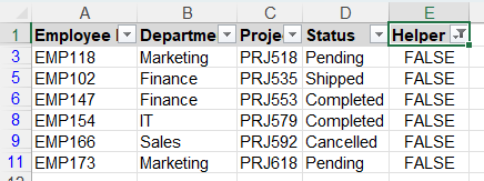
After filtering for FALSE, only unique rows remain visible. All duplicate rows, including their first occurrences, are filtered out and hidden from view.
Pros
- Can hide all duplicate records including first occurrences
- Works in all modern Excel versions
- Easy to customize for one column or multiple columns
Cons
- Requires a helper column
- Additional filtering steps required
Hide duplicates within records that meet specific criteria
Sometimes you may want to hide duplicates only within a specific subset of data. For example, you may want to display unique records from a particular region, department, or product category while ignoring all other records. In this case, you can use Advanced Filter to first filter the data based on your criteria and then display only unique records from the matching results.
Examples:
- Display unique records only for customers in the West region.
- Display unique products only for items with a quantity greater than 50.
- Display unique orders only for records marked as Completed.
In this case, you can use Advanced Filter to filter the data based on your criteria and display only unique records within the filtered result:
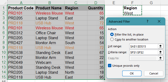
- Prepare a criteria range.
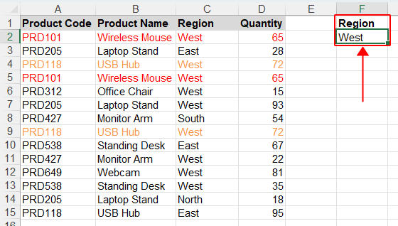
💡 Tip: Make sure the criteria range uses the same headers as the source data. Then enter the condition below the appropriate header.
- Click Data > Advanced.
- Choose Filter the list, in-place.
- In the List range box, select your source data range, including the header row.
- In the Criteria range box, select the criteria range you prepared.
- Check Unique records only.
- Click OK.
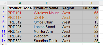
According to your criteria, only the rows that meet the conditions and are unique are visible. Duplicate occurrences are hidden, while the first occurrence is kept visible.
📝 Note:
Advanced Filter keeps the first occurrence of duplicate records visible.
💡 Tip:
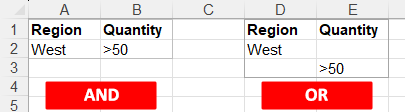
Advanced Filter is a powerful filtering tool that lets you combine duplicate checking with one or more conditions:
- Criteria entered on the same row work as AND conditions.
- Criteria entered on different rows work as OR conditions.
Hide duplicates within filtered subsets
Sometimes duplicates only matter within the currently filtered records. For example, you may filter the data to show only one region, one month, or one product category, and then hide duplicates only within those visible records.
Examples:
- Hide duplicate customers in the West region only.
- Hide duplicate orders for the current month.
- Hide duplicate products within a selected category.
In this situation, you can use a helper column to identify duplicate values among the filtered result:
- Insert a helper column beside the filtered data.
- Enter one of the following formulas:
- To identify duplicate values in Column A within the currently visible rows, excluding the first occurrence:
=IF(SUBTOTAL(103,A2),SUMPRODUCT(SUBTOTAL(103,OFFSET($A$2,ROW($A$2:A2)-ROW($A$2),0)),--($A$2:A2=A2))>1,FALSE) - To identify duplicate values in Column A within the currently visible rows, including the first occurrence:
=SUMPRODUCT(SUBTOTAL(103,OFFSET($A$2,ROW($A$2:$A$100)-ROW($A$2),0)),--($A$2:$A$100=A2))>1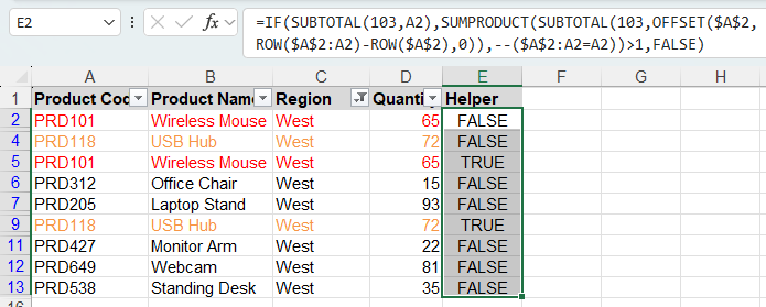
📝 Note:
The formula returns TRUE for rows that belong to a duplicate group, and FALSE for rows that contain unique values only.
- To identify duplicate values in Column A within the currently visible rows, excluding the first occurrence:
- Click To Actual on the Kutools tab to convert the formula results into static values.
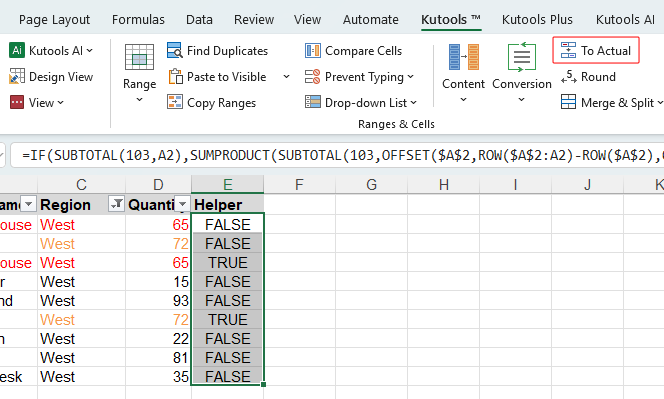
Note:
When a range is filtered, Excel copies only visible cells, which can make it difficult to paste the results back into the original range. Using To Actual avoids this limitation by converting the formulas directly to static values.
- Click Data > Filter.
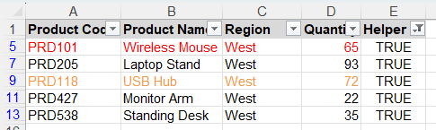
- Filter the helper column:
- Filter for FALSE if you want to hide duplicates and keep only unique visible records.
- Filter for TRUE if you want to review the duplicate records first.
Conclusion
There are several ways to hide duplicates in Excel without deleting the original data. If you only want duplicate values to disappear visually, Conditional Formatting and Kutools' Select Duplicate & Unique Cells are convenient options. To hide entire duplicate rows, Advanced Filter and Kutools' Find Duplicates can quickly display unique records while keeping the first occurrence visible.
If you need more control, such as hiding all duplicate records including the first occurrence or working with specific subsets of data, helper formulas and filtering techniques provide greater flexibility. Choose the method that best fits your dataset and reporting requirements to make duplicate records easier to review and manage.
I hope you found this tutorial helpful. If you’d like to explore more Excel tips and practical solutions, please click here to browse our full collection of Excel tutorials.
The Best Office Productivity Tools
Kutools for Excel - Helps You To Stand Out From Crowd
Kutools for Excel Boasts Over 300 Features, Ensuring That What You Need is Just A Click Away...
Office Tab - Enable Tabbed Reading and Editing in Microsoft Office (include Excel)
- One second to switch between dozens of open documents!
- Reduce hundreds of mouse clicks for you every day, say goodbye to mouse hand.
- Increases your productivity by 50% when viewing and editing multiple documents.
- Brings Efficient Tabs to Office (include Excel), Just Like Chrome, Edge and Firefox.
How to join text from different cells into one cell in Excel?
If you have text spread across multiple cells and want to combine it into one cell, Excel offers simple solutions to accomplish this. You can use the CONCATENATE function to merge text into a single destination cell or opt for advanced tools like Kutools for Excel for more flexibility. This article provides step-by-step methods to handle this task efficiently.

Join text from different cells into one with formulas
Join text from different cells into one with Kutools for Excel
 Join text from different cells into one with formulas

Applying the Concatenate function to join the different cell contents, please do as follows:
1. Enter this formula: =CONCATENATE(A2,"-",B2,"-",C2) into a blank cell next to your data, see screenshot:
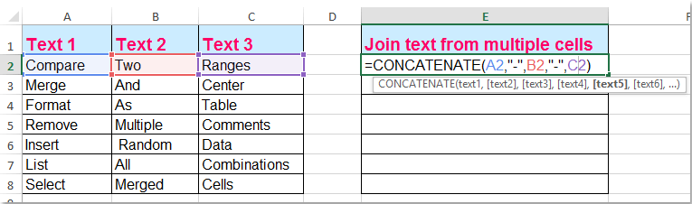
2. Then drag the fill handle down to the cells that you want to join, and the different cells have been merged into one cell by the separator “-”, see screenshot:

Note: If there are more cells needed to be merged together, please join the cell references as this: =CONCATENATE(A2,"-",B2,"-",C2, "-",D2,"-",E2,...), and you can replace the “-” separator in the formula with any character you prefer.
Join text from different cells into one with Kutools for Excel
Kutools for Excel contains a powerful tool - Combine Rows, Columns or Cells without Losing Data. With this utility, you can quickly merge multiple rows, columns, or ranges of cells into one cell using a separator of your choice.
1. Select the text range that you want to join together.
2. Then click Kutools > Merge & Split > Combine Rows, Columns or Cells without Losing Data, see screenshot:

3. In the Combine Columns or Rows dialog box, please do as follows:
(1) Choose one option that you want to join the text based on, you can join cells based on rows, columns or range or just combine all to one single cell;
(2) Specify a separator for your combined data as you need;
(3) Select a location to put the combined result;
(4) At last, choose the option to deal with the combined cells. You can keep or delete contents from those combined cells, and you can also merge those combined cells.

4. After finishing the above settings, click Ok or Apply button, and all the selected text will be combined according to your settings. See screenshot:

Kutools for Excel - Supercharge Excel with over 300 essential tools, making your work faster and easier, and take advantage of AI features for smarter data processing and productivity. Get It Now
Demo: Join text from different cells into one cell in Excel
Best Office Productivity Tools
Supercharge Your Excel Skills with Kutools for Excel, and Experience Efficiency Like Never Before. Kutools for Excel Offers Over 300 Advanced Features to Boost Productivity and Save Time. Click Here to Get The Feature You Need The Most...
Office Tab Brings Tabbed interface to Office, and Make Your Work Much Easier
- Enable tabbed editing and reading in Word, Excel, PowerPoint, Publisher, Access, Visio and Project.
- Open and create multiple documents in new tabs of the same window, rather than in new windows.
- Increases your productivity by 50%, and reduces hundreds of mouse clicks for you every day!
All Kutools add-ins. One installer
Kutools for Office suite bundles add-ins for Excel, Word, Outlook & PowerPoint plus Office Tab Pro, which is ideal for teams working across Office apps.





- All-in-one suite — Excel, Word, Outlook & PowerPoint add-ins + Office Tab Pro
- One installer, one license — set up in minutes (MSI-ready)
- Works better together — streamlined productivity across Office apps
- 30-day full-featured trial — no registration, no credit card
- Best value — save vs buying individual add-in
Table of Contents
- Visually hide duplicate records in a range
- Hide duplicates with Conditional Formatting
- Hide duplicates with Kutools' Select Duplicate & Unique Cells
- Hide duplicate rows
- Hide duplicate rows with Advanced Filter
- Hide duplicate rows with Kutools' Find Duplicates
- Hide duplicate rows including first occurrences with COUNTIF and Filter
- Hide duplicates within records that meet specific criteria
- Hide duplicates within filtered subsets
- Conclusion
- The Best Office Productivity Tools
Kutools for Excel
Brings 300+ advanced features to Excel
- 🧩 Overview
- 📥 Free Download
- 🎁 30-Day Free Trial available