How to hide rows based on cell value in Excel?
When working with large and complex datasets in Excel, it is often necessary to simplify your worksheet so you can better analyze, report, or present the information that matters most. One common need is to hide rows according to specific cell values—such as hiding data entries below a certain threshold or excluding rows that do not meet your criteria. Manually hiding each row can be time-consuming and increases the risk of errors, especially when dealing with hundreds or thousands of entries. In this guide, we’ll demonstrate three practical methods you can use to hide, filter, or selectively manage rows based on cell values in another column. These approaches will help you create tailored views, increase efficiency, and avoid unnecessary manual repetitive tasks.
Hide rows based on cell value with Filter
Excel’s Filter feature is a built-in way to temporarily hide rows according to cell values, making it easy to focus your spreadsheet on the information you need. For example, if you want to display only those sales transactions above $3,000, the Filter tool can instantly help you exclude rows below that amount from view. This approach is most effective for quick manual filtering and when you want to toggle between displaying all data and showing only data that meets certain conditions. It’s simple to use and completely reversible—just remove the filter to restore your original dataset.
Choose this method when you need to filter out data quickly, especially for presentations or iterative analysis, but keep in mind that the rows are only hidden visually; all underlying data remains accessible unless you clear the filter.
1. Select the range of cells or the entire table you want to filter, then click Data > Filter. This will add small filter drop-down arrows to the column headers. See screenshot:

Tip: Make sure no blank rows are in your selection, as this may disrupt filtering for larger data ranges.
2. Click on the drop-down arrow in the target column header to display filter options. Then choose Number Filters (or Text Filters for text-based data) from the menu, and select Greater Than. You can also use other criteria, such as “Less Than”, “Equals”, or “Does Not Equal”, according to your need. See screenshot:

Tip: For text columns, options will include “Contains”, “Begins With”, and similar filters, which can be very useful for non-numeric data.
3. Enter your numeric or text criterion in the textbox next to “is greater than”—for example, type in 3000 to show only values above this amount. See screenshot:

Tip: After typing your criterion, double-check for unwanted spaces or formatting that may affect filtering results.
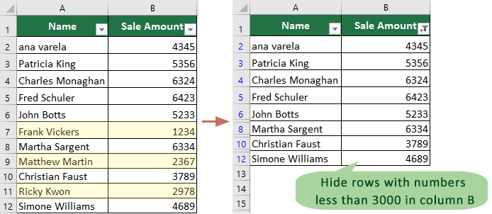
4. Click OK. Now, only the rows with data greater than 3,000 are visible in your worksheet; rows with values less than or equal to 3,000 are hidden from view, though still present in your file. See screenshot:

If you want to restore all rows, simply click the filter icon again and select “Clear Filter from [Column Name]”. Keep in mind that filtered-out rows are only temporarily hidden and not deleted, so any calculations or references to those cells still include them.
Use this solution if you regularly change filter criteria, want quick visual results, or are working collaboratively—since Filter is an Excel standard function, anyone can understand or adjust it.
Drawback: Complex multi-condition filtering or automating repeated custom hide operations may require additional steps or more advanced solutions, such as formulas or VBA.
Quickly select rows based on cell value with Kutools for Excel
For users who need to process large data tables efficiently and often perform batch operations—such as hiding, deleting, or formatting specific rows—Kutools for Excel provides the Select Specific Cells feature to rapidly identify and select all rows that match your chosen cell value criteria. While this feature does not directly “hide” rows, it makes it easy to collectively select target rows, so you can then hide, delete, or format them in one go, greatly speeding up Excel workflow.
This solution is ideal for scenarios where you have complicated criteria, need to select all rows for further processing, or simply want to avoid manual row-by-row selection. Kutools’ approach is very convenient for users dealing with frequent, repetitive tasks and is especially useful for large datasets that standard filtering may not efficiently manage.
After downloading and installing Kutools for Excel, navigate to Kutools > Select > Select Specific Cells to open the Select Specific Cells dialog.
- Select the range: First, highlight the column or area that contains the values you want to use as the selection basis. Ensure your range covers all the relevant rows.
- Choose Entire row: In the Selection type section, select Entire row. This setting allows Kutools to select full rows that meet the criteria, not just the cells.
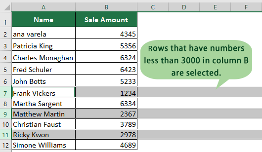
Tip: This is important if you want to hide or process whole data entries, not just individual cells. - Set criteria: In the Specific type drop-down, choose Less than, and enter 3000 in the textbox. This tells Kutools to select all rows where the cell value is less than3,000.
You can also choose “Equal to”, “Greater than”, or “Between”, depending on your filtering needs. - Confirm selection: Click OK to apply the criteria, and Kutools will instantly select the qualifying rows.

Result
All rows containing values less than 3,000 in column B will be automatically selected. These selected rows can then be managed as a group. For example, you can right-click one of the highlighted rows and choose Hide to conceal them, or use other Excel tools for additional batch operations.
Kutools’ solution is recommended for users needing efficiency with large volumes of data, especially when built-in Excel features become too slow or restrictive. The intuitive interface also reduces the risk of selection errors.
Drawback: If you need automatic row hiding based on continuously changing cell values, or if your dataset is very large and updates frequently, consider alternative options such as formulas or VBA code for more dynamic automation.
Hide rows based on cell value with VBA code
If you prefer an automated approach—especially useful when you need to repeatedly hide rows by criteria, or want to integrate row hiding into larger data manipulation tasks—you can use a VBA (Visual Basic for Applications) macro to accomplish this quickly. VBA offers the flexibility to define custom conditions, automate row hiding for large or dynamic datasets, and reduce manual intervention. This method is ideal for advanced Excel users, or anyone needing to perform routine operations across similar spreadsheets.
Pros: The VBA solution enables scalable automation, so you can adjust the criteria or data range easily. It’s very helpful in reports requiring periodic updates, and you can extend or modify the code to adapt to your needs.
Cons: If macros are disabled in your workbook, code will not run; you may need to enable macro security. VBA is more prone to errors from incorrect selection or input, so double-check your steps.
Before running the VBA code, please save your worksheet to prevent any accidental data loss.
1. Press Alt + F11 to open the Microsoft Visual Basic for Applications editor window.
2. In the editor window, click Insert > Module to add a new module to your document. Copy and paste the following VBA code into the module:
VBA: Hide rows based on cell value.
Sub HideRow()
'Updateby20250904
Dim Rng As Range
Dim WorkRng As Range
Dim xNumber As Integer
On Error Resume Next
xTitleId = "KutoolsforExcel"
Set WorkRng = Application.Selection
Set WorkRng = Application.InputBox("Range", xTitleId, WorkRng.Address, Type:=8)
xNumber = Application.InputBox("Number", xTitleId, "", Type:=1)
For Each Rng In WorkRng
    Rng.EntireRow.Hidden = Rng.Value < xNumber
Next
End Sub
3. To run the macro, press F5 or click the Run button. When prompted, select the cell range you wish to process in the pop-up dialog. Be sure to select only the data—not header rows—to avoid hiding column headers inadvertently. See screenshot:

4. Click OK, and after that, a second dialog appears. Enter your criterion number—such as 3000—to specify which rows should be hidden (those below this value). See screenshot:

5. Click OK. The macro will immediately process the selected range, hiding all rows where the value is less than your entered number.
Tip: You can change the logical condition to suit your needs:
- To hide rows with values greater than 3000, update the code in the module to Rng.EntireRow.Hidden = Rng.Value > xNumber.
- To hide rows matching an exact value, modify the code to Rng.EntireRow.Hidden = Rng.Value = xNumber.
If you encounter errors, verify your cell range does not include hidden columns or merged cells, and ensure you have input the correct numerical values. Remember that changes made with VBA are not easily reversible; you may need to unhide rows manually afterward.
For recurring use, you can save this macro for repeated data management tasks, or customize it further (for instance, by adding more complex criteria or supporting text-based conditions).
Hide or flag rows based on cell value with Excel formulas
In addition to the methods above, you can use Excel formulas to help flag or filter rows based on specific cell values, which can then guide you in hiding rows manually or with additional automation tools. This approach is particularly helpful when you want a visual indication (such as a helper column) before hiding, or if you want to sort and group rows for further processing.
For example, you can use a simple formula in a helper column to identify which rows meet your criteria:
1. Enter the following formula in a new column (e.g., column C, cell C2) next to your data:
=IF(B2<3000,"Hide","Show")2. Press Enter, then drag the formula down to fill all rows in your dataset. This marks each row as “Hide” if the cell value is less than 3,000, or “Show” otherwise.
3. You can now use Excel's Filter feature on this helper column to display only rows marked “Show”, or sort your data accordingly. Alternatively, use conditional formatting to highlight “Hide” rows, making manual editing faster.
This formula approach is best when you want to make your criteria visible directly in the sheet, or set up further automation with Kutools or VBA.
Drawback: You still need to manually hide rows based on the formula result, but it helps clarify and reduce mistakes, making batch operations easier.
If you experience issues, such as rows not hiding as expected, check for merged cells, blank rows, or formulas that may interfere with manual or automated selection. Always save before running macros or batch operations. For very large datasets, consider optimizing your Excel file or using helper columns for clarity. Whenever possible, document your methods so collaborators can follow along and maintain consistency in future analysis.
Hide Rows Based on Cell Value
Best Office Productivity Tools
Supercharge Your Excel Skills with Kutools for Excel, and Experience Efficiency Like Never Before. Kutools for Excel Offers Over 300 Advanced Features to Boost Productivity and Save Time. Click Here to Get The Feature You Need The Most...
Office Tab Brings Tabbed interface to Office, and Make Your Work Much Easier
- Enable tabbed editing and reading in Word, Excel, PowerPoint, Publisher, Access, Visio and Project.
- Open and create multiple documents in new tabs of the same window, rather than in new windows.
- Increases your productivity by 50%, and reduces hundreds of mouse clicks for you every day!
All Kutools add-ins. One installer
Kutools for Office suite bundles add-ins for Excel, Word, Outlook & PowerPoint plus Office Tab Pro, which is ideal for teams working across Office apps.
- All-in-one suite — Excel, Word, Outlook & PowerPoint add-ins + Office Tab Pro
- One installer, one license — set up in minutes (MSI-ready)
- Works better together — streamlined productivity across Office apps
- 30-day full-featured trial — no registration, no credit card
- Best value — save vs buying individual add-in