How to quickly flip data upside down in Excel?

In many data management and analysis tasks in Excel, you might encounter situations where the order of your data needs to be reversed—flipping it upside down. This is especially useful when working with time-series datasets, logs, or when you need to compare data trends in opposite directions. Additionally, data imported from various sources might sometimes be in reverse order from what your analysis or reporting format requires. In these cases, quickly inverting the order of your data ensures consistency and accuracy for subsequent processing or visualization.

This comprehensive guide introduces several practical methods to flip data upside down in Excel, including:

Flip data upside down with help column and Sort

One straightforward technique involves using a helper column alongside your data, then sorting based on this helper to systematically reverse the order. This approach is easy to implement and works for both small lists and lengthy datasets.

1. Click the cell directly adjacent to your first data entry. Enter 1 in this helper column cell. In the cell below, input 2. 

2. Highlight the two numbered cells you just entered. Use the autofill handle (the small square at the cell’s lower-right corner) to drag the fill sequence down alongside your data, making sure to match the length of your data range. This action assigns helper numbers sequentially aligned with each data row.

3. With both your data and the full sequence of helper numbers selected, go to the Data tab, and click Sort Largest to Smallest. This will allow you to rearrange the rows so that the data order is inverted according to the helper column.

4. A Sort Warning dialog may appear. Be sure to choose Expand the selection and then click Sort. This ensures the sort operation includes all related columns and preserves the integrity of your data while reversing its order.

Now, the data—including both your helper column and main column—has been reversed in place.

Once finished, you can safely delete or hide the helper column if you no longer need it.

Flip data upside down with formula

For those comfortable with Excel formulas, there’s a quick way to flip a column using an INDEX and ROWS formula. This is ideal for dynamically flipping data without altering the source column. The formula solution is especially practical when you need to keep the original data intact and want the flipped data to update automatically if the source changes.

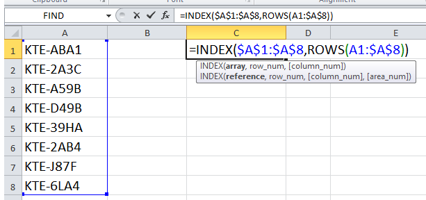
1. In a blank column (for example, if your original data is in A1:A8, start in cell B1), input this formula:

=INDEX($A$1:$A$8,ROWS(A1:$A$8))

2. Press Enter. Then, drag the formula’s autofill handle down through as many rows as your original data range covers, until the data is reversed. Once duplicate entries start to appear, stop filling further rows.

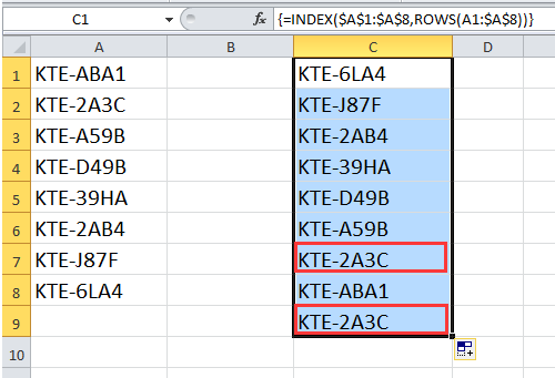
Now your data will display upside down in the new column while the source remains unchanged.

Parameter explanation: INDEX($A$1:$A$8,ROWS(A1:$A$8)) pulls data from A8 to A1 successively. Adjust $A$1:$A$8 to your actual data range.

Flip data upside down with Kutools for Excel

While the standard Excel methods above reverse the order of values, sometimes you also need to preserve cell formatting, such as background colors, fonts, or data validation. In these cases, Kutools for Excel’s "Flip Vertical Range" utility delivers added flexibility, allowing you to flip both values and formatting together, or just values if preferred.

After installing Kutools for Excel, select the data you wish to flip. Navigate to Kutools > Range > Flip Vertical Range, and then specify your preferred flip type from the submenu.

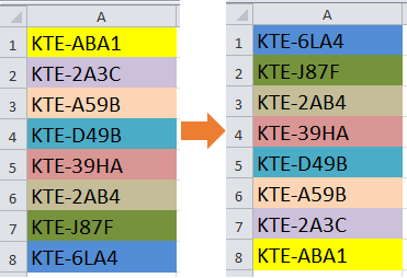
• If you choose Flip All, both cell values and corresponding formats are reversed simultaneously. The output will look like this:
  
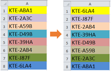
• If you choose Only flip values, only content values are inverted while formatting remains unchanged:
  

Kutools for Excel not only helps with flipping data and formats but also offers numerous utilities for swapping ranges, batch editing, and improving efficiency in complex data scenarios.

Scenario advantages and cautions: This approach is highly recommended for users who routinely manipulate data layouts or need to preserve complex cell styles. The operation is direct and reduces the risk of manual error. However, this solution requires Kutools for Excel to be installed. As with any add-in, always keep a backup of important data before performing batch transformations.

Flip data upside down with VBA code 

If you frequently need to reverse large datasets or automate the flipping process, using a VBA macro can help streamline your workflow. This method is particularly valuable for those managing repetitive tasks or dealing with very large datasets, as the macro will flip the range quickly and consistently with a single execution. It’s also useful when incorporating the flip operation into a broader automated data-processing task.

1. On the Excel Ribbon, go to Developer > Visual Basic to open the Microsoft Visual Basic for Applications window. In the project pane, click Insert > Module, then paste the following VBA code into the new module:

Sub FlipDataUpsideDown()
    Dim WorkRng As Range
    Dim i As Long, j As Long
    Dim TempValue As Variant, TempFormat As Variant
    
    On Error Resume Next
    xTitleId = "KutoolsforExcel"
    
    Set WorkRng = Application.Selection
    Set WorkRng = Application.InputBox("Please select the range to flip upside down:", xTitleId, WorkRng.Address, Type:=8)
    
    If WorkRng Is Nothing Then Exit Sub
    
    Application.ScreenUpdating = False
    
    For i = 1 To Int(WorkRng.Rows.Count / 2)
        j = WorkRng.Rows.Count - i + 1
        TempValue = WorkRng.Rows(i).Value
        TempFormat = WorkRng.Rows(i).Interior.Color
        WorkRng.Rows(i).Value = WorkRng.Rows(j).Value
        WorkRng.Rows(i).Interior.Color = WorkRng.Rows(j).Interior.Color
        WorkRng.Rows(j).Value = TempValue
        WorkRng.Rows(j).Interior.Color = TempFormat
    Next i
    
    Application.ScreenUpdating = True
End Sub

2. Then, click the Run button to execute the code. A dialog will prompt you to select the range you wish to flip upside down. After confirming your selection, the chosen cells will automatically have their order reversed vertically. The macro also copies cell background colors during the flip.

With the range of methods introduced in this guide—manual helper column and sorting, formula-based solutions, Kutools for Excel utilities, and customizable VBA macros—you can confidently reverse data order in Excel to suit countless business and analytical scenarios. When choosing a method, consider the size of your data, your comfort level with Excel functions and code, and whether you need to retain cell formatting. If errors or unexpected results occur, double-check your data selection steps, range references, and restore from backup if necessary.

Mastering these data manipulation skills greatly enhances your ability to adapt Excel spreadsheets to your exact workflow needs, helping you work faster, reduce the risk of mistakes, and gain deeper insights from your data. For additional tips, formulas, and automation ideas, visit our Excel resources section for more step-by-step tutorials.

Flip Data Vertically or Horizontally