How to split a column every other row in Excel?
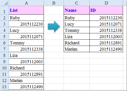
When working with long lists in Excel, you may encounter scenarios where you need to divide a single column into two separate columns, with each new column containing every other row from the original list. For instance, if you have a contact list or a series of transaction records, and you wish to alternate rows to create two balanced lists, this task can be a bit tricky to execute manually, especially with large data sets. The screenshot illustrates this challenge, where data from a single column is split into two columns by alternating rows. Efficiently managing this operation ensures that your data organization becomes much clearer and can be tailored for further analysis or reporting.
There are several practical approaches available to address this in Excel, each suitable for different preferences and needs:
In the following sections, you'll find detailed step-by-step guides for using formulas, applying a VBA macro, and utilizing the Kutools for Excel utility to achieve the desired result. Additionally, practical tips, precautions, and troubleshooting advice are included to help you avoid common pitfalls and ensure a smooth process regardless of which method you choose.
Split a column every other row with Formula
Using formulas is a straightforward method for splitting one column into two columns by every other row. This technique is particularly effective when you need a dynamic solution that automatically updates when source data changes, or when you want to avoid using macros or add-ins.
Below are the steps to apply the formulas to achieve this split:
1. Enter the following formula into a blank cell—for example, cell C2. This formula extracts every odd row (the 1st, 3rd, 5th, etc.) from your source data range (here, $A$2:$A$13):
=INDEX($A$2:$A$13,ROWS(C$1:C1)*2-1)This formula works by using the ROWS function to calculate the position in the list and multiplies by2, then subtracts1 to get odd-numbered rows only.
For example, when you enter this formula in C2 and drag down, you'll get entries from A2, A4, A6, etc.

2. After entering the formula, drag the fill handle down the column until you see error values such as #REF!. These errors appear when the formula tries to reference rows outside your specified range, indicating you have reached the end of your data. It's recommended to stop dragging when the last valid value appears and remove error cells afterward for a cleaner result.

3. In cell D2, enter the next formula to extract every even row (2nd, 4th, 6th, etc.) from your source range:
=INDEX($A$2:$A$13,ROWS(D$1:D1)*2)Drag this formula down the D column in the same manner. It returns A3, A5, A7, etc. as you fill downward.
If necessary, remove any error values at the end for neatness.

Applicable scenarios for the formula solution include regular lists where the number of rows is even, or where you are comfortable deleting any extra error values. If your list contains blank rows, note that these will also be transferred according to their position; you should check for unintended gaps after the split.
Tips & Precautions: Make sure cell references are adjusted to match your actual data range. If the source data size changes, re-check your formulas as errors may occur. Also, when dragging the formula, ensure that you do not extend past your intended data set.
- If you encounter #REF! errors, it means the formula is trying to select a row beyond your source range. You can hide these errors by using an
IFERRORwrapper, for example:=IFERROR(INDEX($A$2:$A$13,ROWS(C$1:C1)*2-1),"")This variant will display blank cells instead of error codes, creating a cleaner final output, especially when presenting results to others. - If you are using Excel 365 or Excel 2021 and above, the newer FILTER and SEQUENCE functions can automate the split in dynamic tables. You can create two ranges using formulas like:
=FILTER(A2:A100,MOD(SEQUENCE(ROWS(A2:A100)),2)=1)for odd rows.=FILTER(A2:A100,MOD(SEQUENCE(ROWS(A2:A100)),2)=0)for even rows.
Split a column every other row with VBA code
If you prefer automation and have a larger dataset, or regularly perform this task, a VBA macro can efficiently split a column into two by alternating rows. VBA is suitable for situations where you want more control or need to customize the process for various data sizes.
Follow these steps to use the VBA solution:
1. In Excel, hold down ALT + F11 to open the Microsoft Visual Basic for Applications editor window.
2. Click Insert > Module to bring up a blank coding pane, then copy and paste the following code into the Module window:
VBA code: Split a column into two columns every other row
Sub SplitEveryOther()
'Updateby Extendoffice
Dim Rng As Range
Dim InputRng As Range, OutRng As Range
Dim index As Integer
xTitleId = "KutoolsforExcel"
Set InputRng = Application.Selection
Set InputRng = Application.InputBox("Range :", xTitleId, InputRng.Address, Type:=8)
Set OutRng = Application.InputBox("Out put to (single cell):", xTitleId, Type:=8)
Set OutRng = OutRng.Range("A1")
num1 = 1
num2 = 1
For index = 1 To InputRng.Rows.Count
    If index Mod 2 = 1 Then
        OutRng.Cells(num1, 1).Value = InputRng.Cells(index, 1)
        num1 = num1 + 1
    Else
        OutRng.Cells(num2, 2).Value = InputRng.Cells(index, 1)
        num2 = num2 + 1
    End If
Next
End Sub 3. Press F5 to execute the macro. A prompt box will appear, asking you to select the data range you want to split. Choose your target cells, then click OK.

4. Next, a second prompt asks you to select a starting output cell where the split results will be placed. Specify a vacant cell as the beginning of your output range to prevent overwriting any existing data.

5. After clicking OK, the macro will split your original column into two columns, alternating rows, starting from your designated output cell. Review the output for completeness and accuracy.

Pros of this VBA solution include speed and automation, especially for repetitive tasks or larger datasets. However, users should save their work before running macros, as VBA actions may overwrite data if the output cell is not carefully chosen. If you experience errors or unexpected results, double-check your selected ranges and review whether merged cells or hidden rows could affect the outcome.
Tip: If your dataset contains formulas or special formatting, note that the macro copies only the displayed values and does not transfer cell formatting. Adjust accordingly as needed after the split.
Split a column every other row with Kutools for Excel
If you are looking for a more efficient approach without using formulas or VBA, Kutools for Excel offers a convenient way to split a column every other row. Its Transform Range utility simplifies the process, making it ideal for users who prefer graphical interfaces and want quick results without manual configuration.
Once Kutools for Excel is installed, carry out the following steps:
1. Select your columnar data in Excel that you want to split into two columns alternating every other row. Ensure that there are no merged cells or hidden rows within the selection for best results.
2. On the ribbon, go to Kutools > Range > Transform Range. This will open the utility dialog box.

3. In the Transform Range dialog, select Single column to range under Transform type. In the Rows per record section, choose Fixed value and enter 2. This setting tells Kutools to organize every two rows into one horizontal record (which can be interpreted as one row per column split).

4. Click the Ok button. You will be prompted to select a cell where you want the split results to appear. Choose a target cell that is empty to avoid overwriting any existing content.

5. Click OK once more. The utility will instantly split your selected list into two columns by every other row.
Click to know more about this Transform Range utility.
Kutools for Excel's solution is suitable for users who want a hassle-free method and frequently handle tasks like data reshaping or row-to-column conversions. Its design makes it especially useful for those uncomfortable writing formulas or VBA code.
Precaution: Before confirming the output cell, always check if there is enough space for the results. If the original list is long, outputting the split data over existing cells could cause data loss.
Kutools for Excel - Supercharge Excel with over 300 essential tools, making your work faster and easier, and take advantage of AI features for smarter data processing and productivity. Get It Now
Troubleshooting & Summary Suggestions: If your split results are incorrect, double-check your selection ranges and formula references. Also, verify if your original data contains blank cells, merged cells, or formatting that could affect splitting. Always back up your original data before performing any VBA operations or using add-ins like Kutools. When using formula solutions, wrap with IFERROR for cleaner outputs. For large lists or recurring tasks, consider automating with VBA or using Kutools for maximum efficiency.
Best Office Productivity Tools
Supercharge Your Excel Skills with Kutools for Excel, and Experience Efficiency Like Never Before. Kutools for Excel Offers Over 300 Advanced Features to Boost Productivity and Save Time. Click Here to Get The Feature You Need The Most...
Office Tab Brings Tabbed interface to Office, and Make Your Work Much Easier
- Enable tabbed editing and reading in Word, Excel, PowerPoint, Publisher, Access, Visio and Project.
- Open and create multiple documents in new tabs of the same window, rather than in new windows.
- Increases your productivity by 50%, and reduces hundreds of mouse clicks for you every day!
All Kutools add-ins. One installer
Kutools for Office suite bundles add-ins for Excel, Word, Outlook & PowerPoint plus Office Tab Pro, which is ideal for teams working across Office apps.
- All-in-one suite — Excel, Word, Outlook & PowerPoint add-ins + Office Tab Pro
- One installer, one license — set up in minutes (MSI-ready)
- Works better together — streamlined productivity across Office apps
- 30-day full-featured trial — no registration, no credit card
- Best value — save vs buying individual add-in