How to filter data by multiple colors in Excel?
In regular Excel usage, applying a filter based on cell color is straightforward when dealing with a single color. However, what if you need to filter rows containing more than one specific color at the same time? For example, suppose you have a data list formatted with several categories highlighted with different fill colors, and you need to view only the rows containing two or more selected colors. This scenario cannot be handled directly through Excel’s standard filtering features since the built-in filter only allows one color choice at a time. This article introduces efficient methods for solving this problem and explains their practical value and situations where you might prefer one approach over another.
Below you will find the VBA code solution originally presented, along with extra tips and cautions to help you get the best results. In addition, you'll find two alternative methods (using helper columns with formulas and the Kutools for Excel add-in) linked for your convenience:
Filter data by multiple colors with VBA code
Manually categorize and filter data by multiple colors in Excel
 Filter data by multiple colors with VBA code
Currently, Excel does not offer a native way to filter rows based on more than one cell background color at the same time. When you need to display only rows matching several specific colors, you can turn to a customized VBA solution. The approach below demonstrates how to use a user-defined function to extract color index numbers into an adjacent helper column. After identifying the colors this way, you can filter as needed using Excel’s built-in filter tools. This method works best for small to moderately sized data sets, and it is particularly helpful if you’re comfortable using macros.
1. Hold down the ALT + F11 keys to open the Microsoft Visual Basic for Applications window. If you want to keep the code in your workbook for future use, save the file as a macro-enabled workbook (.xlsm) or another format that supports macros, since regular Excel files (.xlsx) cannot store VBA code.
2. Click Insert > Module, and paste the following code into the open Module window.
VBA code: Extract color index number:
Function GetColor(x As Range) As Integer
GetColor = x.Interior.ColorIndex
End Function
Before you continue, ensure you have saved your work. Using VBA will prompt a security warning in some cases, so enable macros if prompted.
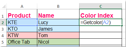
3. Return to your worksheet. Next to your data, select a blank cell (for example, if your colored cells are in column A and your first row of data is row2, use B2), and enter the formula: =Getcolor(A2). Here, A2 refers to the first colored cell you want to analyze. This function will return the color index as a number into the helper column. See screenshot:

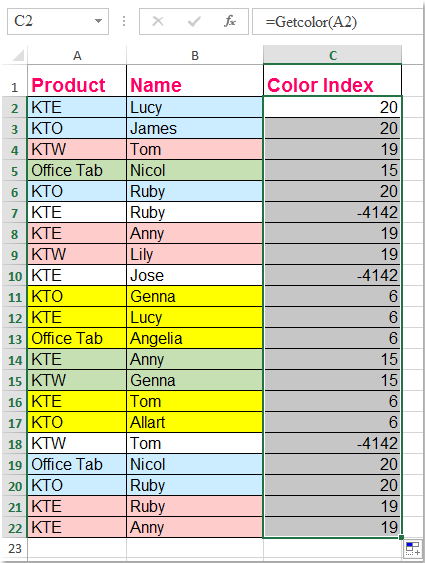
4. Use the fill handle to copy this formula down alongside your data range, so every row now shows the color index for that row. If your table is large, you can double-click the fill handle to fill the column to match your data automatically. All rows will now display a color index number, as shown below:

Tips: If a cell doesn't have any background color, the function will return -4142. You may use this as a reference if you want to exclude rows without color.
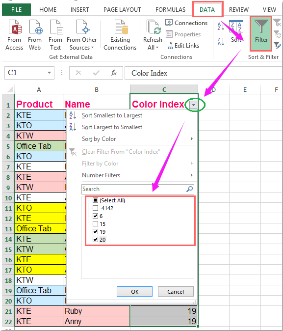
5. Now that each row is associated with a specific color index, you can filter your data to show only the rows with the desired colors. To do this, select your helper column, go to the Data tab, click Filter, and then click the arrow at the top of the helper column. In the filter dropdown list, check the boxes for all the color index numbers corresponding to the colors you wish to display, as shown here:

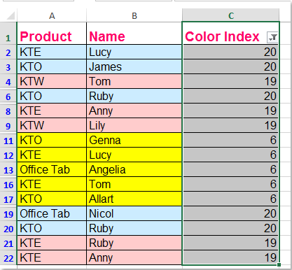
6. Click OK to apply the filter. Only rows with the selected background colors will now be displayed in your data range. If you wish to further analyze or copy the results, you can select the filtered rows. See screenshot:

7. Lastly, if you no longer need the helper column visible, you can safely hide or delete it. Just be aware that deleting the column after filtering will remove its color references if you try to re-filter, so it's best to hide it unless you're finished with this analysis.
If you get the #NAME? error after entering the formula, it's likely that the VBA code is not properly inserted, or macros are not enabled. Double-check your VBA module and macro security settings.
One of the advantages of this solution is that it lets you combine color-based filtering with other types of criteria, such as text or value filters, using Excel’s native filter controls. However, a limitation is that cell color codes may change if you apply a new theme or copy data from other sources, which may require you to refresh or reapply the VBA function.
Manually categorize and filter data by multiple colors in Excel
If employing VBA doesn’t suit your needs due to workbook security policies or user preferences, a practical workaround involves manually coding the color categories in a helper column, then filtering based on those categories. This solution is suitable for situations where the number of distinct colors is manageable and adjustments to the color codes are infrequent.
You can create a helper column (e.g., “Color Category”) next to your data and manually assign a label to each row according to its fill color (e.g., “Red,” “Green,” “Yellow”). Then, use the filter feature to display only the categories you wish to see.
Steps: In your helper column, enter simple text identifiers based on the color (for instance, “Blue” for blue-filled rows, “None” for no fill). Once completed, select the helper column and use Data > Filter to choose any combination of colored rows for display.
This approach is less automatic but gives you more flexibility if your data set is small or if color definitions tend to change. If your data is dynamically changing or used by different users, manual maintenance may be less efficient.
For large data sets or frequent updates, consider automating this process with VBA or using a specialized Excel add-in as introduced below.

Unlock Excel Magic with Kutools AI
- Smart Execution: Perform cell operations, analyze data, and create charts—all driven by simple commands.
- Custom Formulas: Generate tailored formulas to streamline your workflows.
- VBA Coding: Write and implement VBA code effortlessly.
- Formula Interpretation: Understand complex formulas with ease.
- Text Translation: Break language barriers within your spreadsheets.
Related articles:
How to filter comma separated data in Excel?
How to filter exact text in Excel?
Best Office Productivity Tools
Supercharge Your Excel Skills with Kutools for Excel, and Experience Efficiency Like Never Before. Kutools for Excel Offers Over 300 Advanced Features to Boost Productivity and Save Time. Click Here to Get The Feature You Need The Most...
Office Tab Brings Tabbed interface to Office, and Make Your Work Much Easier
- Enable tabbed editing and reading in Word, Excel, PowerPoint, Publisher, Access, Visio and Project.
- Open and create multiple documents in new tabs of the same window, rather than in new windows.
- Increases your productivity by 50%, and reduces hundreds of mouse clicks for you every day!
All Kutools add-ins. One installer
Kutools for Office suite bundles add-ins for Excel, Word, Outlook & PowerPoint plus Office Tab Pro, which is ideal for teams working across Office apps.
- All-in-one suite — Excel, Word, Outlook & PowerPoint add-ins + Office Tab Pro
- One installer, one license — set up in minutes (MSI-ready)
- Works better together — streamlined productivity across Office apps
- 30-day full-featured trial — no registration, no credit card
- Best value — save vs buying individual add-in