How to transpose reference while auto fill down/right in Excel?

When working with formulas and autofill in Excel, the default behavior is for column references to increment as you drag the fill handle horizontally to the right, and for row references to increment as you drag vertically downward. However, sometimes you may need to transpose references — for instance, referencing a vertical range but filling horizontally, or vice versa. This operation is especially useful when reorganizing data layouts or building dynamic reports that require cross-referencing data in transposed fashions. This article will explore various practical methods to achieve this transposed autofilling, including formulas, VBA macros, and convenient tools like Kutools. See the illustration below for a typical transposed autofill scenario:

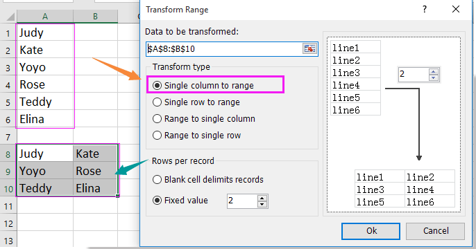
Transpose reference while fill down or right

Excel Formula – Use INDEX or OFFSET to manually construct transposed references

Transpose reference while fill down or right

To transpose a reference while filling across rows or columns, the TRANSPOSE function in Excel can be utilized. This method is suitable when you want to convert data that is arranged in a column into a row (or vice versa), with the formula automatically adjusting the direction of the reference as you autofill.

Select the range where you'd like to apply the transposed reference. Enter the following formula in the formula bar: =TRANSPOSE(Sheet2!$B$1:B12) and then press Ctrl + Shift + Enter simultaneously (for versions earlier than Microsoft 365 / Excel 2021). In new versions that support dynamic arrays, simply pressing Enter is sufficient.See the screenshot below:

In this formula, B1:B12 represents the range you wish to transpose from a vertical range to a horizontal arrangement. You can adjust the sheet name and the specific range to fit your actual data source.
Tip: To avoid formula errors, ensure the destination range for the transposed data is sized appropriately (e.g., if your source is one column with 12 rows, your destination range should be one row with 12 columns).

Tip. If you want to quickly convert a range to a single column or row (or vice versa) many times, or if the ranges are large and formulas become unwieldy, you can efficiently accomplish this using Kutools for Excel’s Transform Range utility. This tool offers a straightforward interface and flexibility for transforming ranges, minimizing the risk of formula errors or mismatches. The feature is fully functional for 60 days. Please download and try it for free.

Excel Formula – Use INDEX or OFFSET to manually construct transposed references

Sometimes using array formulas like TRANSPOSE is not preferred, or you require more control over how references are transposed, especially for non-contiguous data or when working in older Excel versions. With INDEX and OFFSET functions, you can reference transposed data directly using standard fill operations, without needing Ctrl + Shift + Enter.

Applicable Scenarios: Preferable when you want a one-to-one transposed reference per cell, for example, referencing cell A1 vertically to B1 horizontally (or vice versa). Useful for avoiding array entries, or for dynamic references across complex worksheets.

Advantages: No array input required, formulas are simple to drag-and-fill.
Potential drawbacks: Can be a bit more involved to set up initial formula; pay close attention to how you adjust row and column indices.

How to use INDEX for transposed referencing:

1. Suppose you have data in A1:A5 (vertical), and you want to fill it transposed in B1:F1 (horizontal). Select cell B1 and enter the following formula:

=INDEX($A$1:$A$5,COLUMN(A1))

2. Press Enter, then drag the formula to the right up to cell F1. The formula uses COLUMN(A1) to increment as you move right, thus referencing A1, A2, ..., A5 across B1:F1.

How to use OFFSET for transposed referencing:

1. Suppose your data is in row B1:F1 (horizontal), and you want to fill it vertically down column G1:G5. In cell G1, enter:

=OFFSET($B$1,0,ROW(A1)-1)

2. Press Enter, then drag the formula down to G5. As you fill down, ROW(A1)-1 will increment from 0, shifting the column index of the OFFSET function to fetch B1, C1, D1, etc.

Adjust the formula range or starting position as needed to match your data layout. Always verify correct referencing, especially when copying or moving formulas, to avoid reference mismatches.

Troubleshooting: If you get a #REF! error, double-check the reference ranges and ensure the formula is not trying to reference outside your target data set. Also, for large datasets, these formulas can increase workbook calculation load.

In summary, whether you choose to use formulas, VBA, or an Excel add-in depends on your data structure, the frequency with which you need to perform this operation, and your comfort level with advanced Excel features. If one approach doesn't fit your needs, try another method as described above. If you encounter persistent formula or reference issues, double-check your formulas for locked cell references (use of $ symbols) and adjust as necessary for correct directionality when transposing.

Unlock Excel Magic with Kutools AI

• Smart Execution: Perform cell operations, analyze data, and create charts—all driven by simple commands.
• Custom Formulas: Generate tailored formulas to streamline your workflows.
• VBA Coding: Write and implement VBA code effortlessly.
• Formula Interpretation: Understand complex formulas with ease.
• Text Translation: Break language barriers within your spreadsheets.

Enhance your Excel capabilities with AI-powered tools. Download Now and experience efficiency like never before!