How to filter data from drop down list selection in Excel?
In Excel, many users are familiar with filtering data using the standard Filter feature. However, there are times when you may want to filter or display data interactively using a drop-down list selection. For example, you might need rows of data to update dynamically and display only information that matches what you've selected from a drop-down menu, as shown in the screenshot below. This approach enables more user-friendly reports, dashboards, and interactive forms. This article covers several practical methods to filter or visually highlight data based on drop-down list selections in one or two worksheets, offering you flexible options suited for different needs.

Filter data from drop down list selection in one worksheet with helper formulas
Filter data from drop down list selection in two worksheets with VBA code
Conditional Formatting - Highlight rows matching the drop down selection
Filter data from drop down list selection in one worksheet with helper formulas
To filter data based on a drop-down list, you can set up a series of helper columns using formulas to create a dynamic extraction of matching rows. This method is ideal when you want to show only the relevant records on the same worksheet, without using macros. Follow these steps:
1. Begin by inserting the drop-down list. Select the cell where you want the drop-down, then navigate to Data > Data Validation > Data Validation. This step creates a cell where users can pick an item to filter by.

2. In the Data Validation dialog box under the Settings tab, select List from the Allow drop down, then click the  button to highlight the range of values for your drop-down list. Using a named range or table for the list source can help keep lists updated automatically later.

3. Once your drop-down list is set, choose any item to filter. In cell D2, enter the following formula (assuming your drop-down selection is in column H):
=ROWS($A$2:A2)Here, A2 refers to the first cell in the column containing data to be matched. Drag the fill handle downwards to fill for all relevant rows. This helper column generates row sequence numbers, making it easier to reference rows later.

4. Next, in cell E2, enter:
=IF(A2=$H$2,D2,"")This formula checks if the value in A2 matches the selected drop-down item in H2. If it matches, it outputs the row number from D2; otherwise, it leaves the cell blank. This is a crucial filtering step: make sure your drop-down cell reference (here H2) does not change unexpectedly.

5. In cell F2, input:
=IFERROR(SMALL($E$2:$E$17,D2),"")This formula extracts the row numbers of filtered data, allowing you to later return the corresponding entries. Be sure the range E2:E17 covers all your filtered formula cells. Extend the fill handle down as needed.

6. To display the filtered results, enter the following formula in cell J2:
=IFERROR(INDEX($A$2:$C$17,$F2,COLUMNS($J$2:J2)),"")Copy this formula from J2 to L2 to display the first matching record. This step uses the results of your helper columns to retrieve the actual data rows based on the drop-down selection. Adjust columns if your original data uses a different range.

Note: A2:C17 is your original table, F2 is the filtered helper column, J2 is where you want the output to appear.
7. Drag the fill handle down all output columns to display every matching record.

8. Now, whenever you select an item from the drop-down list, the table below updates dynamically to only show rows that match the selection.

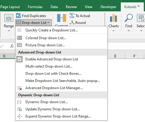
Supercharge Excel Dropdown Lists with Kutools Enhanced Features
Elevate your productivity with Kutools for Excel's enhanced dropdown list capabilities. This feature set goes beyond basic Excel functionalities to streamline your workflow, including:
- Multi-select Dropdown List: Select multiple entries simultaneously for efficient data handling.
- Dropdown List with Check Boxes: Enhance user interaction and clarity within your spreadsheets.
- Dynamic Dropdown List: Automatically updates based on data modifications, ensuring accuracy.
- Searchable Dropdown List: Quickly locate needed entries, saving time and reducing hassle.
Filter data from drop down list selection in two worksheets with VBA code
Sometimes, you may need to filter data in one worksheet after selecting an item from a drop-down list located in a different worksheet. For example, Sheet1 contains the selection, and Sheet2 holds the table to filter. In such cases, using VBA is a practical solution as formulas can't directly update other sheets in response to an event. This approach suits dashboards, reports, or summary workbooks where data sources and user inputs are separated for clarity.
1. Right click the sheet tab (e.g., Sheet1) with the drop-down cell, choose View Code. In the Microsoft Visual Basic for Applications window, copy and paste the following code into the blank Module:
VBA code: Filter data from drop down list selection in two sheets:
Private Sub Worksheet_Change(ByVal Target As Range)
'Updateby Extendoffice
    On Error Resume Next
    If Not Intersect(Range("A2"), Target) Is Nothing Then
        Application.EnableEvents = False
        If Range("A2").Value = "" Then
            Worksheets("Sheet2").ShowAllData
        Else
            Worksheets("Sheet2").Range("A2").AutoFilter 1, Range("A2").Value
        End If
        Application.EnableEvents = True
    End If
End Sub
Note: In the code, A2 refers to the drop-down cell, Sheet2 is where the filter occurs, and AutoFilter 1 designates the column for filtering. Adjust these based on your data layout. Make sure worksheet and cell names are consistent with your actual structure to avoid runtime errors. If you encounter unexpected behavior, check for sheet protection, merged cells, or hidden data that can interfere with the AutoFilter method.

2. Now, selecting any drop-down item in Sheet1 immediately filters the data in Sheet2, making analysis across worksheets seamless for reporting and reviewing.

Note that VBA-based solutions require Macros to be enabled. Always save your workbook as an .xlsm file if you want the code to persist. If your filter does not update, review macro security settings and ensure the references and worksheet names match. Avoid using sensitive or business-critical data without proper backup, as macros can make bulk changes.
Conditional Formatting - Automatically highlight all rows matching the drop down selection
If your goal is not to hide or extract rows, but simply to visually highlight which ones match the drop-down selection, Conditional Formatting provides a fast, user-friendly approach. Use this when you want users to focus on relevant lines without removing or moving data.
The most common use is in dashboards, reports, or large lists where highlighting instantly shows which entries relate to the current choice, improving data readability.
- Select your data range: For example, select A2:C100.
- Access the Conditional Formatting tool: Go to Home > Conditional Formatting > New Rule.
- Create your rule: Choose Use a formula to determine which cells to format, and enter a formula like:
This highlights any row where the value in column A matches the drop-down selection in H2.=$A2=$H$2 - Set the formatting: Click Format, then choose a fill color or text format. Press OK to confirm.
Advantages: quick setup, works instantly as selections change, and does not disrupt table structure. However, this only highlights (does not filter or extract) records. For large tables, use high-contrast colors to ensure highlighted rows are noticeable. Conditional Formatting rules are cell-based—if cell references are wrong, not all rows may highlight as expected. Use absolute references (like $H$2) in your formula for consistency.
If you want to remove highlighting, just go to Conditional Formatting > Clear Rules. For multi-condition or multi-column highlights, adjust your formula to check more columns or use the AND function.
Best Office Productivity Tools
Supercharge Your Excel Skills with Kutools for Excel, and Experience Efficiency Like Never Before. Kutools for Excel Offers Over 300 Advanced Features to Boost Productivity and Save Time. Click Here to Get The Feature You Need The Most...
Office Tab Brings Tabbed interface to Office, and Make Your Work Much Easier
- Enable tabbed editing and reading in Word, Excel, PowerPoint, Publisher, Access, Visio and Project.
- Open and create multiple documents in new tabs of the same window, rather than in new windows.
- Increases your productivity by 50%, and reduces hundreds of mouse clicks for you every day!
All Kutools add-ins. One installer
Kutools for Office suite bundles add-ins for Excel, Word, Outlook & PowerPoint plus Office Tab Pro, which is ideal for teams working across Office apps.
- All-in-one suite — Excel, Word, Outlook & PowerPoint add-ins + Office Tab Pro
- One installer, one license — set up in minutes (MSI-ready)
- Works better together — streamlined productivity across Office apps
- 30-day full-featured trial — no registration, no credit card
- Best value — save vs buying individual add-in