How to vlookup to return multiple columns from Excel table?
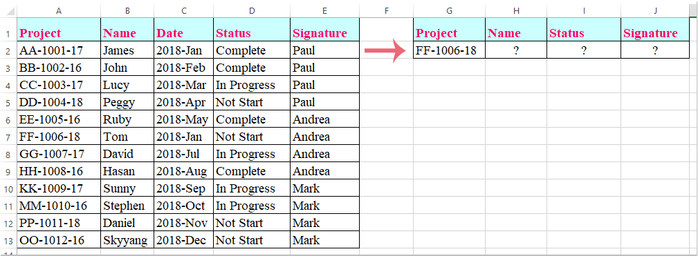
In Excel worksheet, you can apply the Vlookup function to return the matching value from one column. But, sometimes, you may need to extract matched values from multiple columns as following screenshot shown. How could you get the corresponding values at the same time from multiple columns by using the Vlookup function?
Vlookup matching values from multiple columns with array formula
Vlookup matching values from multiple columns with array formula
Here, I will introduce the Vlookup function to return matched values from multiple columns, please do as this:
1. Select the cells where you want to put the matching values from multiple columns, see screenshot:

2. Then enter the following formula into the formula bar, and then press Ctrl + Shift + Enter keys together, and the matching values form multiple columns have been extracted at once, see screenshot:
=VLOOKUP(G2,A1:E13,{2,4,5},FALSE)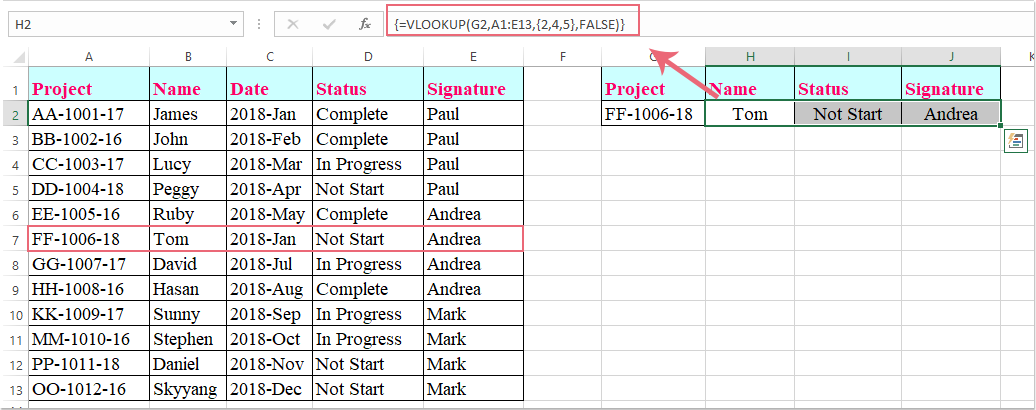
Note: In the above formula, G2 is the criteria that you want to return values based on, A1:E13 is the table range you want to vlookup from, the number 2, 4, 5 are the column numbers which you want to return values from.
Overcome VLOOKUP Limits with Kutools: Super LOOKUP
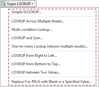
To address the limitations of the VLOOKUP function in Excel, Kutools has developed multiple advanced LOOKUP features, offering users a more powerful and flexible data lookup solution.
- 🔍 LOOKUP Across Multiple Sheets...: Perform lookups across multiple worksheets to find matching data.
- 📝 Multi-condition Lookup...: Search for data that meets multiple criteria simultaneously.
- ➕ LOOKUP and Sum...: Search for data based on a lookup value and sum the results.
- 📋 One-to-many Lookup (returns multiple results)...: Retrieve multiple matching values for a single lookup input.
- Get Kutools For Excel Now!
Best Office Productivity Tools
Supercharge Your Excel Skills with Kutools for Excel, and Experience Efficiency Like Never Before. Kutools for Excel Offers Over 300 Advanced Features to Boost Productivity and Save Time. Click Here to Get The Feature You Need The Most...
Office Tab Brings Tabbed interface to Office, and Make Your Work Much Easier
- Enable tabbed editing and reading in Word, Excel, PowerPoint, Publisher, Access, Visio and Project.
- Open and create multiple documents in new tabs of the same window, rather than in new windows.
- Increases your productivity by 50%, and reduces hundreds of mouse clicks for you every day!
All Kutools add-ins. One installer
Kutools for Office suite bundles add-ins for Excel, Word, Outlook & PowerPoint plus Office Tab Pro, which is ideal for teams working across Office apps.
- All-in-one suite — Excel, Word, Outlook & PowerPoint add-ins + Office Tab Pro
- One installer, one license — set up in minutes (MSI-ready)
- Works better together — streamlined productivity across Office apps
- 30-day full-featured trial — no registration, no credit card
- Best value — save vs buying individual add-in